 2022, Vol. 40
Institute of Oceanology, Chinese Academy of Sciences
Article Information
- HE Qiu, TIAN Fenglin, YANG Xiaokun, CHEN Ge
- Lagrangian eddies in the Northwestern Pacific Ocean
- Journal of Oceanology and Limnology, 40(1): 66-77
- http://dx.doi.org/10.1007/s00343-021-0392-7
Article History
- Received Oct. 16, 2020
- accepted in principle Nov. 23, 2020
- accepted for publication Jan. 9, 2021


2 Laboratory for Regional Oceanography and Numerical Modeling, Pilot National Laboratory for Marine Science and Technology (Qingdao), Qingdao 266237, China;
3 Key Laboratory of Urban Land Resources Monitoring and Simulation, Ministry of Natural Resources, Shenzhen 518034, China
Time mean flow is generally considered the main carriers of energy and materials in the western Pacific Ocean. The Kuroshio Current is the strongest time mean flow in this region, with a maximum volume transport of 100 Sv or more (Hasunuma and Yoshida, 1978; Mizuno and White, 1983; Qiu and Chen, 2005). However, previous studies show that transport by mesoscale eddies cannot be neglected. Mesoscale eddies are an important component of ocean dynamic systems, and they transport more materials and energy in the ocean than the time mean flow (Chelton et al., 2007, 2011b). Zhang et al. (2014) found that volume transport was 500–1 000 Sv or greater in the Northwest Pacific. Dong et al. (2014) reported results that were roughly within this scale. With the development of remote sensing technology, the detection of mesoscale eddies based on sea surface height (SSH) is widely used (Chelton et al., 2011a). Generally, many mesoscale eddies can be identified using remote sensing data of the sea surface at a certain time. Previous work showed that the mesoscale eddies identified in SSH fields corresponded with distinct mesoscale features that were identified using in-situ hydrography (Yang et al., 2013; Liu et al., 2016; Xu et al., 2016). The abilities of different eddies to package and transport materials differ significantly. Eddies with a stable and strong core can isolate the internal and external material as much as possible and may have stronger volume transport. Therefore, a stricter mesoscale eddy definition is needed to identify eddies with an effective transport capacity and improve the accuracy of the analytical results. This method should be different from the previous method that first identifies the eddy then tracks it. Lagrangian eddies have time coherence, which more accurately describes the transport of matter (Wang et al., 2016).
The Lagrangian coherent structure (LCS) approach provides a means of identifying key material lines that organize fluid-flow transport. More specifically, the LCS approach is based on the identification of material lines that play the dominant role in attracting and repelling neighboring fluid elements over a selected period. It was frequently used for material structure extraction and analysis to study and predict a variety of ocean phenomena (Peacock and Haller, 2013). Different from other methods based on instantaneous flow fields, Lagrangian eddies are surrounded by closed material boundaries (Blazevski and Haller, 2014). This method describes a coherent and stable material structure and defines the transport capacity of mesoscale eddies. Mesoscale eddy recognition based on the LCS allows us to focus more on its transport function. Beron-Vera et al. (2015) used the correlation method to evaluate the material transport on the Agulhas circulation and the Gulf of Mexico. Hadjighasem and Haller (2014) also used this method to identify the red spot on Jupiter. In contrast to structures identified using Eulerian eddy-tracking methods, the Lagrangian eddies maintain material coherence over the specified time intervals, which makes them suitable for material transport estimates. Lagrangian eddies and SSH eddies propagate westward at similar speeds at each latitude, which is consistent with the Rossby wave dispersion relationship. However, the Lagrangian eddies are uniformly smaller and shorter-lived than SSH eddies (Abernathey and Haller, 2018). The present study used the null-geodesic Lagrangian eddy extraction method for the western Pacific Ocean over the past 20 years. The fast calculation of Lagrangian eddies was realized. Section 2 introduces the related research background in recent years. Section 3 details the data and data processing methods used in the present paper. We discuss the seasonal variation, secular variation, and material transport capacity of the Lagrangian eddy in Section 4. The spatial and temporal distributions of the Lagrangian eddy are examined, and the transport capacity was evaluated quantitatively. Finally, the conclusion is provided in Section 5.
2 RELATED WORKThe spatial distribution of mesoscale eddies in the Northwest Pacific is not uniform. These eddies are more likely to occur in mid latitudes, especially in the Kuroshio extension (Chelton et al., 2007; Yang et al., 2013; Ding et al., 2020). This type of distribution law widely exists in the same types of sea areas worldwide. There are nonnegligible large-scale long-term changes over time in addition to seasonal periodic changes (Lin et al., 2020; Sun et al., 2020). Lin et al. (2020) and Ding et al. (2018) showed that the large-scale decadal Pacific modes, such as the North Pacific Gyre Oscillation (NPGO), was the reason for these long-term changes. It affected the surrounding environment via the transportation of materials and energy such as temperature, salinity, etc. (Zhang et al., 2019, 2020). For example, the distribution of chlorophyll and storm track were closely related to the changes of eddy (Lin et al., 2014, 2019).
Haller and Yuan (2000) coined the LCS acronym to describe the most repelling, attracting, and shearing material surfaces that form the skeleton of Lagrangian particle dynamics. First, some methods, including Finite-Time Lyapunov Exponent/Finite-Size Lyapunov Exponent (FTLE/FSLE), appeared, but these methods are not sufficiently accurate and objective and are not suitable for the detection of elliptic (eddy-type) LCSs in finite-time flow data (Haller and Beron-Vera, 2012; Harrison et al., 2013).
To accurately define the LCS, Haller and Beron-Vera (2012) introduced the variational geodesic theory of LCSs. The geodesic theory of LCSs is a collection of global variational principles for material surfaces that form the centrepieces of coherent, time-evolving tracer patterns (Haller and Beron-Vera, 2012; Haller, 2015). The geodesic LCS theory is objective because it builds on material notions of strain and shear that are expressible through the invariants of the right Cauchy-Green strain tensor, which makes the LCS more widely usable in fluid structure extractions and analyses (Onu et al., 2015). We generally refer to closed shear lines as elliptic LCSs and consider the outermost member of a nested elliptic LCS family to be the boundary of a coherent Lagrangian eddy (Haller and Beron-Vera, 2013; Haller, 2015), which allows LCSs to accurately describe the mesoscale eddy in an incompressible two-dimensional flow field. Other Lagrangian eddy extraction methods, such as the Lagrangian averaged vorticity deviation (LAVD), were proposed recently (Haller et al., 2016).
Lagrangian eddy boundaries are sought as closed stationary curves of the averaged Lagrangian strain. Solutions to this problem turn out to be mathematically equivalent to photon spheres around black holes in cosmology (Haller and Beron-Vera, 2013; Huhn et al., 2015). Relevant methods are widely applied in marine data analyses, for example, the assessment and prediction of material transport in the Atlantic circulation and South Atlantic circulation (Wang et al., 2015) and attempting to identify the Great Red Spot (Hadjighasem and Haller, 2014). Recent results suggest that the boundaries of coherent fluid eddies (elliptic coherent structures) were identified as closed null geodesics of the appropriate Lorentzian metrics defined in the flow domain. Mattia Serra derived an automated method for computing the null geodesics based on the geometry of the underlying geodesic flow (Hadjighasem et al., 2017; Serra and Haller, 2017; Aksamit et al., 2019). This method showed that coherent mesoscale Lagrangian eddies, which were detected earlier in mesoscale-resolving ocean data only, continue to persist with the addition of energetic submesoscale velocity features (Haller et al., 2018; Beron-Vera et al., 2019; Katsanoulis et al., 2020).
3 DATA AND METHOD 3.1 DataWe apply the two-dimensional unsteady ocean flow dataset obtained from AVISO Maps of Sea Level Anomaly (MSLA) and geostrophic velocity data from 1998–2019 (AVISO Satellite Altimetry Data, 2020). The temporal resolution with geostrophic velocities is 1 day, and the spatial resolution is 1/4 degrees. The temporal resolution of the chlorophyll data is also 1 day, but the spatial resolution is 1/24 degrees. The El Niño phenomenon was obtained from the National Climate Center (National Climate Centre, 2020). A study area from 100°E–180°E, 0°–50°N is selected, and Fig. 1a shows the extent of the region and the results of Lagrangian eddy identification on January 1, 2018. As a comparison, SSH eddy data from AVISO (NRT 3.0exp product) is used in Fig. 1b showing 331 SSH eddies and 165 Lagrangian eddies. Their average diameters are 163 km and 95 km, respectively. The number of perfect matching is 90, accounting for 55% of Lagrangian eddy and 27% of SSH eddy.

|
| Fig.1 Lagrangian eddies in the western Pacific Ocean on January 1, 2018 a. the color of the base map represents the sea level anomaly (SLA) value. The black solid line represents an anticyclone eddy, and the grey line represents a cyclone eddy; b. comparison between Lagrangian eddy and SSH eddy including cyclone and anticyclone. |
Lagrangian coherent eddies, in the sense of, are encircled by elliptic LCSs, i.e., exceptional material barriers that exhibit no appreciable stretching or folding over a finite time interval. Here we derive an automated method for computing such null geodesics based on the geometry of the underlying geodesic flow. Our approach simplifies and improves existing procedures for computing variationally defined Lagrangian eddy boundaries (Serra and Haller, 2017).
For an unstable two-dimensional flow field,
 (1)
(1)where U represents the range of the flow field region, and x represents the velocity of the flow field. Then, the positional change in the particle in this period can be defined as follows:
 (2)
(2)Based on the mapping relationship between displacement and time interval, the Lagrangian variation can be described by the Cauchy-Green strain tensor:
 (3)
(3)The Cauchy-Green strain tensor is second order in a two-dimensional flow field. It describes the force and movement trend of particles in fluid. The eigenvalues and eigenvectors are described as follows:
 (4)
(4)For the boundary of the Lagrangian eddy, the Lorentz quantity is described as follows:
 (5)
(5)λ is a constant here to express the different values of the stretching rate. For a given time interval [t0, t1] and lambda value, the elliptic LCS satisfies the following point-by-point condition:
 (6)
(6)According to the above methods, we synchronously adopt the parallel acceleration technology based on a graphics processing unit (GPU), which improves the original calculation efficiency by approximately 20–30 times. For example, the calculation in our study area generally requires more than 10 h in previous methods, but now 20 min is adequate (personal computer with Intel Core i7-8700 CPU and NVIDIA GeForce GTX 1060 3GB). Therefore, it is possible to consider the long-term Lagrangian eddies in the western Pacific. Specifically, we transplant the algorithm to the python environment and use the Numba library to call the CUDA core of NVIDIA graphics card to speed up the calculation. The accelerated part is concentrated in the array operation section.
4 RESULT AND DISCUSSIONUsing global MSLA data from 1998 to 2018, we extract Lagrangian eddies in the western Pacific Ocean. The spatial and temporal distributions of the Lagrangian eddy in this region are inhomogeneous. We calculate the frequency of the Lagrangian eddy in the region at different times to show our results directly. The study area is divided into 1°×1° grids. Each eddy belongs to different region according to the position of eddy centre, and will be calculated only once. Figure 2 shows the average number of times the region is affected by eddies (diameter > 50 km) each month. Some small eddies can be filtered out from the restriction of diameter, while their credibility is low, so as to better highlight the distribution differences between different areas.

|
| Fig.2 The occurrence frequency of Lagrangian eddy with diameter greater than 50 km The color in the figure represents the frequency at which the area falls into the eddy region each month. |
The average number of simultaneous Lagrangian eddies in our selected region is 181 per day. The average diameter of all eddies is 91.7 km. The frequencies of eddies in summer and autumn are lower than those in spring and winter. The distribution is concentrated mainly in the mid-latitude region but less concentrated in the tropical region. There are almost no Lagrangian eddies in the regions near the equator, which is consistent with the previous understanding of the distribution of mesoscale eddies (Abernathey and Haller, 2018). Simultaneously, we note that there is an eddy vacuum zone of long-term existence in the mid-latitude region, i.e., 30°N–40°N. This zone may exist because the Kuroshio extension is located in this area, and the widespread strong current affects the generation of Lagrangian eddies (Hogan and Hurlburt, 2000; Kouketsu et al., 2012).
The high incidence areas of eddies are concentrated in the Japan Sea and on both sides of the Kuroshio extension. There are many reasons for the high occurrence of eddies in the Japan Sea, among which the complex submarine topography is very important. A large amount of warm water is injected from the south of the Tsushima Strait and mixed with the local cold water, which promotes formation of the eddy. In the southern part of the Japan Sea, the interlaced basins and ridges divide this area into several independent regions and mesoscale eddies develop independently in each basin. As a result, there are many small but stable mesoscale eddies in this region. The depth of the vast Japan Basin reaches 3 500 m in the northern part of the Japan Sea, which makes eddy generation difficult (Hogan and Hurlburt, 2000). In the Sea of Japan, the number of eddies identified is not more than that of Chelton et al. (2007) (Fig. 1). The reason for our results is that most of the SSH eddies in this area are considered to be Lagrangian eddies, while many SSH eddies in other areas are not. This shows that although the size of the eddy is small and the amplitude is weak, eddies in the Sea of Japan have strong encapsulation and has a certain ability to carry material. The topography is no longer the main cause of eddies on both sides of the Kuroshio extension. The Kuroshio brings much warm water from the tropical area to meet the cold water in the north, which forms an ocean front that aggravates the disturbance of sea water and promotes eddy generation. A large amount of kinetic energy carried by the Kuroshio is also consumed here, and some of the energy is transferred to eddies. For example, some eddies are shed from the Kuroshio extension.
The diameter of the Lagrangian eddy is generally approximately 50–200 km, and smaller Lagrangian eddies are rare. This rarity may be due to our limited data resolution, which makes it impossible to extract smaller-scale eddies. The maximum size of the Lagrangian eddy is lower than our previous understanding of the mesoscale eddy, which is also mentioned by Abernathey and Haller (2018). This difference occurs because the boundary of the Lagrangian eddy must be a barrier to material transport and block the flow and exchange of materials on both sides of the eddy. It is the traditional definition of an eddy boundary, which is stricter and more accurate. However, it also reduces the boundary size of the eddy.
4.1 The seasonal variation in the Lagrangian eddyLagrangian eddies in the western Pacific region have a periodic occurrence pattern characterized by the appearance of more eddies in spring and fewer in autumn. These characteristics are shown in Fig. 3. The reason for this phenomenon may be the large temperature difference in the upper layer of the North Pacific Ocean in spring and summer, which is more unstable and prone to eddies when a disturbance occurs. Su et al. (2018) also showed a periodic oscillation in the global scale.

|
| Fig.3 The annual average number of Lagrangian eddies in the western Pacific The black solid line represents the total number of vortices; the blue and yellow lines represent the number of cyclones and anticyclones, respectively. |
To further examine this periodic oscillation, we classify the identified Lagrangian eddies according to size. The large and small eddies are larger than 150 km and smaller than 50 km in diameter, respectively, and the medium eddies are between 50–150 km in diameter. According to this classification, Fig. 3 is refined to Fig. 4. The distributions of mid-sized eddies below 50–150 km and small eddies below 50 km are greater in spring and fewer in autumn, respectively. This result is identical to the general rule obtained previously. However, the seasonal cycle of large eddies greater than 150 km is contrary to the overall law, with fewer in spring and more in autumn. This finding is beyond our expectation. However, because less than 20% of the Lagrangian eddies are large eddies, the influence on the general law is very small. It is difficult to say that the opposite is due to the size of the eddy. Because the larger eddies are mostly distributed in the low latitude area, this phenomenon may also be due to latitude differences.

|
| Fig.4 The annual average number of Lagrangian eddies of different sizes in the western Pacific From (a) to (c): the sizes correspond to large (diameter > 150 km), medium (150 km > diameter > 50 km), and small (diameter < 50 km), respectively. |
The Lagrangian eddies also have secular variation. There is a correlation between the eddy number and the strength of the El Niño. We introduce the El Niño coefficient to describe the strength of the El Niño phenomenon.
Table 1 shows the relationship between the Lagrangian eddy number and the El Niño coefficient for different months. Here, we calculate the number of daily average eddies per month from 1999 to 2018. The covariance between the average numbers and the three kinds of Niño coefficients is obtained. Observation revealed that the number of Lagrangian eddies lags the El Niño coefficient. Therefore, we list the results when the Lagrangian eddies match their corresponding El Niño coefficients for the previous months. The results show that the number of eddies in the selected region has an obvious response to different El Niño coefficients, but different Niño coefficients have different response intensities and response times. There is a positive correlation between them, especially when the eddies lag by 3–7 months.
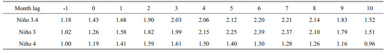
Figure 5 shows the El Niño coefficient of 3.4 to describe this hysteresis. The two groups of parameters have a high correlation after normalization. An obvious lag exists between these factors. There are obvious peaks in the El Niño coefficient in 2009 and 2015, which are well matched with the number of eddies. The general correlation of other years is also consistent, but the two parameters do not necessarily keep up with the fine changes and individual months.

|
| Fig.5 Secular variation in Lagrangian eddies with El Niño 3.4 a. the original diagram of the relationship between the number of eddies and the Niño coefficient; b. the results after translating the folding line of eddies for 7 months. The red solid line represents the trend of the El Niño coefficient of 3.4. The black solid line represents the trend of eddy numbers in the study area from 1998 to 2018. |
These correlation studies examine the study area as a whole. Therefore, we study the interannual correlation between the number of Lagrangian eddies and the El Niño coefficient in different regions to obtain new results. Figure 6 shows the correlation of these different regions. There is an obvious positive correlation between the variation in the Lagrangian eddies and the El Niño coefficient in most regions of the study area. However, there is an area under the Kuroshio extension between 20°N–30°N that exhibits the opposite relationship. This phenomenon is similar under the three El Niño coefficients.

|
| Fig.6 The effect of different regions on the El Niño coefficient a. El Niño 3.4; b. El Niño 3; c. El Niño 4. |
To measure the contributions of Lagrangian eddies to material transport, we divide them into cyclonic eddies and anticyclonic eddies according to the direction of flow velocity and used the centre of the boundary mass as the centre of eddies. After superimposing the same type of Lagrangian eddy, the surrounding chlorophyll situation is shown in Fig. 7.

|
| Fig.7 The results of chlorophyll abnormalities caused by normalized eddies show that yellow is positive and blue is negative a. for the anticyclone Lagrangian eddy, there was downwelling in the center, which led to a cavity in the eddy center; b. for the cyclonic Lagrangian eddy, the upwelling in the center increased the chlorophyll concentration. |
To ensure the accuracy and objectivity of the results, we eliminate the eddies near the continental shelf. The abnormal chlorophyll signal caused by eddies in this area is inconspicuous and distorted. Figure 7 shows the normalized chlorophyll concentrations of the anticyclone (Fig. 7a) and cyclonic (Fig. 7b) Lagrangian eddies (radius > 50 km). Only eddies with radii greater than 50 km are selected mainly because the smaller eddy has less influence on the surrounding area, and it is difficult to produce an obvious chlorophyll abnormality. Due to the large difference in eddy sizes, we scale the radius to the same value to improve the normalization effect. We observe obvious chlorophyll holes and aggregation centres. These results demonstrate that the Lagrangian eddy has a strong wrapping property for the water mass, which indicates that the properties in the centre are significantly different from the properties around the eddy. The normalized core in Fig. 7a is more complete than that in Fig. 7b, and there is a gap in the low chlorophyll concentration on the left side of Fig. 7b. Some reasons for this phenomenon are described as follows. First, the cold eddy has a longer existence time than the warm eddy, and there is sufficient time for chlorophyll to respond to the change in water mass. Second, the chlorophyll concentration is affected by sunlight and other factors, and the transport effect of eddies cannot fully explain the pattern. Notably, on the edges of Fig. 7, the chlorophyll concentration is opposite to the centre. The dipole effect or the nearby upwelling/downwelling may be the cause of this phenomenon. The normalized core in Fig. 7a is more complete than that in Fig. 7b, and there is a gap in the low chlorophyll concentration on the left side of Fig. 7b.
We quantitatively describe the material transport capacity of the Lagrangian eddy in the Northwest Pacific. It is helpful to understand the contribution of mesoscale eddies to material transport. Due to the lack of three-dimensional eddy data, we can only assume an ideal three-dimensional model of eddies, where the cross-sectional area decreases downward from the sea surface (Zhang et al., 2014). We assume that the influential depth of the eddy with the same area as that of the standard eddy with a radius of 100 km is 1 000 m. Due to the lack of three-dimensional data support, we can only estimate the depth of the Lagrangian eddy. In a similar study, the influence depth of 1 km is used to calculate the transport capacity of the Lagrangian eddy (Beron-Vera et al., 2019). In the papers of Zhang et al. (2014) and Dong et al. (2014), the fixed depth of 2 km and the standard eddy model are selected respectively. Therefore, we finally give the plan in this paper that is generally reasonable. We may be conservative in some sense, but it has limited impact on the subsequent analysis. The influential depth of other eddies is scaled according to the ratio of their area to the standard eddy area. Equation 7 describes the calculation process of transport volume:
 (7)
(7)where S is the volume of an eddy, and d and v are its diameter and velocity, respectively. Therefore, VT is the transport volume of an eddy. The average transport volume of eddies VT can be obtained by summing the transport volume and averaging the total number of days identified.
The effect of mesoscale eddies on material transport is different by region. Figure 8 shows the distribution of the transport capacity of the Lagrangian eddy in the study area. We divide the study area into grids, calculate the average transport volume of eddies in the grid, divide the results by the grid area, and obtain the average transport volume per unit area, which makes the average transport intensity and direction of the Lagrangian eddies obvious. Because most mesoscale eddies generally propagate westward, the transport direction of Lagrangian eddies is mainly westward. The six main black curves represent the path of eddy transport (Fig. 8). Except for the corridor near 35°N, the eddies are transported westward. The path of the South China Sea is special and is affected by topography, first to the west and then to the south.

|
| Fig.8 Average transport intensity of Lagrangian eddies in the Northwest Pacific The blue and white areas represent areas with high and low traffic volumes, respectively. The large yellow arrows indicate the main transport corridors of Lagrangian eddies. A–D and F depict five west direction transport channels, while only E is heading east. These six transport channels are the main long-lived material transport channels in the Northwest Pacific region. |
Figure 9 shows the detailed variation in the Lagrangian eddy transport in the study area. Figure 9a–b calculates the average transport volume of eddies meridionally and by latitude, respectively. Latitudinal transport is stronger generally than meridional transport. We decompose the total transport into the cyclonic contribution and anticyclone contribution (red line and blue line, respectively). The results show that their contributions to transport are quite different. Cyclonic eddies tend to dominate meridional transport, and anticyclones dominate zonal transport. However, there are some exceptions. For example, extremely strong eastward cyclones dominate the direction and intensity of transport near 35°N. The lettering in Fig. 9 corresponds to the letters in Fig. 8. The five transport extremes in Fig. 9a represent the B–F transport corridors in Fig. 8. Only channel E is eastward, which is related to the local strong cyclonic eddies. The eastward flow of the Kuroshio extension also affects the direction of the eddy in this area. Channel A is seen as an obvious meridional transport corridor in Fig. 9b. A distinct southward transport appears near 110°E, which proves the existence of channel A.

|
| Fig.9 Variation in the mean Lagrangian eddy transport in the Northwest Pacific a. eddy-induced zonal transport through meridional cross section per degree of latitude; b. eddy-induced meridional transport through a zonal cross section per degree of longitude. The red and blue lines are the cyclonic and anticyclonic components. The black line represents the sum of the above two. The vertical column symbols show the local extremum of transport, which represent the main transport channels. A–F corresponds to the transport channels in Fig. 8. |
The transport volume of the mesoscale eddy is westward in the mass in the Northwest Pacific. In summary, the latitudinal direction is stronger than the meridional direction, the western direction is stronger than the eastern direction, and the northern direction is stronger than the southern direction. The total transport volume is several times larger than that of the Kuroshio Current. The real-time Lagrangian eddy identification method is more conservative than the traditional eddy identification method, and the difference in transport volumes is also very large. However, the transport of mesoscale eddies is not as continuous and directional as the Kuroshio because its existence is unstable.
5 CONCLUSIONMesoscale eddies play an important role in the transport of materials in the ocean, especially when there is no obvious ocean current as the main body of transport. Previous studies of the Lagrangian eddy were very limited in time and space due to the calculation conditions. We improve the original calculation method of the Lagrangian eddy and realize a continuous parallel based on the GPU, which improves the computational efficiency by several times. We identify the Lagrangian eddies in the western Pacific region over 20 years, which makes it possible to analyse secular variations.
The present paper describes the spatial and temporal distributions of the Lagrangian eddy, and its periodic oscillation in a year is determined. The eddies extracted with the Lagrangian method conform to the general law of periodic variation in mesoscale eddies. The relationship between the number of Lagrangian eddies and the El Niño phenomenon is described quantitatively. This finding shows that the Lagrangian eddy has secular variations and is closely related to El Niño and other climatic phenomena. Unfortunately, we cannot predict this change, just as we cannot predict El Niño.
The Lagrangian eddy boundary based on closed zero geodesics effectively identifies the material transport boundary of mesoscale eddies, which lays the foundation for the measurement of the material transport capacity of mesoscale eddies. Our assessment of material transport is bound to be conservative because Lagrangian eddies are smaller than other eddies in terms of quantity and single area. In the future, we need more data and a more detailed evaluation to discuss the transport capacity of the Lagrangian eddy in different sea areas and at different times.
6 DATA AVAILABILITY STATEMENTThe El Niño data are obtained from the National Climate Center (https://cmdp.ncc-cma.net/pred/cn_enso.php?product=cn_enso_nino_indices). The datasets generated and analyzed during the current study are available from the corresponding author on reasonable request.
Abernathey R, Haller G. 2018. Transport by lagrangian vortices in the eastern Pacific. Journal of Physical Oceanography, 48(3): 667-685.
DOI:10.1175/JPO-D-17-0102.1 |
Aksamit N O, Sapsis T P, Haller G. 2019. Machine-learning ocean dynamics from lagrangian drifter trajectories. arXiv preprint arXiv: 1909.12895.
|
AVISO Satellite Altimetry Data. 2020. Gridded sea level heights and derived variables. https://www.aviso.altimetry.fr/index.php?id=1271. Accessed on 2020-10-10.
|
Beron-Vera F J, Hadjighasem A, Xia Q, Olascoaga M J, Haller G. 2019. Coherent lagrangian swirls among submesoscale motions. Proceedings of the National Academy of Sciences of the United States of America, 116(37): 18251-18256.
DOI:10.1073/pnas.1701392115 |
Beron-Vera F J, Olascoaga M J, Haller G, Farazmand M, Triñanes J, Wang Y. 2015. Dissipative inertial transport patterns near coherent lagrangian eddies in the ocean. Chaos: An Interdisciplinary Journal of Nonlinear Science, 25(8): 087412.
DOI:10.1063/1.4928693 |
Blazevski D, Haller G. 2014. Hyperbolic and elliptic transport barriers in three-dimensional unsteady flows. Physica D: Nonlinear Phenomena, 273-274: 46-62.
DOI:10.1016/j.physd.2014.01.007 |
Chelton D B, Gaube P, Schlax M G, Early J J, Samelson R M. 2011a. The influence of nonlinear mesoscale eddies on near-surface oceanic chlorophyll. Science, 334(6054): 328-332.
DOI:10.1126/science.1208897 |
Chelton D B, Schlax M G, Samelson R M, de Szoeke R A. 2007. Global observations of large oceanic eddies. Geophysical Research Letters, 34(15): L15606.
|
Chelton D B, Schlax M G, Samelson R M. 2011b. Global observations of nonlinear mesoscale eddies. Progress in Oceanography, 91(2): 167-216.
DOI:10.1016/j.pocean.2011.01.002 |
Ding M R, Lin P F, Liu H L, Chai F. 2018. Increased eddy activity in the northeastern Pacific during 1993-2011. Journal of Climate, 31(1): 387-399.
DOI:10.1175/JCLI-D-17-0309.1 |
Ding M R, Lin P F, Liu H L, Hu A X, Liu C Y. 2020. Lagrangian eddy kinetic energy of ocean mesoscale eddies and its application to the northwestern Pacific. Scientific Reports, 10(1): 12791.
DOI:10.1038/s41598-020-69503-z |
Dong C M, McWilliams J C, Liu Y, Chen D K. 2014. Global heat and salt transports by eddy movement. Nature Communications, 5(1): 3294.
DOI:10.1038/ncomms4294 |
Hadjighasem A, Farazmand M, Blazevski D, Froyland G, Haller G. 2017. A critical comparison of Lagrangian methods for coherent structure detection. Chaos: An Interdisciplinary Journal of Nonlinear Science, 27(5): 053104.
DOI:10.1063/1.4982720 |
Hadjighasem A, Haller G. 2014. Geodesic transport barriers in Jupiter's atmosphere: a video-based analysis. SIAM Review, 58(1): 69-89.
|
Haller G, Beron-Vera F J. 2012. Geodesic theory of transport barriers in two-dimensional flows. Physica D: Nonlinear Phenomena, 241(20): 1680-1702.
DOI:10.1016/j.physd.2012.06.012 |
Haller G, Beron-Vera F J. 2013. Coherent lagrangian vortices: the black holes of turbulence. Journal of Fluid Mechanics, 731: R4.
DOI:10.1017/jfm.2013.391 |
Haller G, Daniel K, Florian K. 2018. Material barriers to diffusive and stochastic transport. Proceedings of the National Academy of Sciences of the United States of America, 115(37): 9074-9079.
DOI:10.1073/pnas.1720177115 |
Haller G, Hadjighasem A, Farazmand M, Huhn F. 2016. Defining coherent vortices objectively from the vorticity. Journal of Fluid Mechanics, 795: 136-173.
DOI:10.1017/jfm.2016.151 |
Haller G, Yuan G. 2000. Lagrangian coherent structures and mixing in two-dimensional turbulence. Physica D: Nonlinear Phenomena, 147(3-4): 352-370.
DOI:10.1016/S0167-2789(00)00142-1 |
Haller G. 2015. Lagrangian coherent structures. Annual Review of Fluid Mechanics, 47: 137-162.
DOI:10.1146/annurev-fluid-010313-141322 |
Harrison C S, Siegel D A, Mitarai S. 2013. Filamentation and eddy-eddy interactions in marine larval accumulation and transport. Marine Ecology Progress Series, 472: 27-44.
DOI:10.3354/meps10061 |
Hasunuma K, Yoshida K. 1978. Splitting of the subtropical gyre in the western North Pacific. Journal of Oceanography, 34(4): 160-172.
DOI:10.1007/BF02108654 |
Hogan P J, Hurlburt H E. 2000. Impact of upper ocean-topographical coupling and isopycnal outcropping in Japan/East Sea models with to  to to  resolution. Journal of Physical Oceanography, 30(10): 2535-2561.
DOI:10.1175/1520-0485(2000)030<2535:IOUOTC>2.0.CO;2 resolution. Journal of Physical Oceanography, 30(10): 2535-2561.
DOI:10.1175/1520-0485(2000)030<2535:IOUOTC>2.0.CO;2 |
Huhn F, van Rees W M, Gazzola M, Rossinelli D, Haller C, Koumoutsakos P. 2015. Quantitative flow analysis of swimming dynamics with coherent lagrangian vortices. Chaos: An Interdisciplinary Journal of Nonlinear Science, 25(8): 087405.
DOI:10.1063/1.4919784 |
Katsanoulis S, Farazmand M, Serra M, Haller G. 2020. Vortex boundaries as barriers to diffusive vorticity transport in two-dimensional flows. Physical Review Fluids, 5(2): 024701.
DOI:10.1103/PhysRevFluids.5.024701 |
Kouketsu S, Tomita H, Oka E, Hosoda S, Kobayashi T, Sato K. 2012. The role of meso-scale eddies in mixed layer deepening and mode water formation in the western north pacific. Journal of Oceanography, 68(1): 63-77.
DOI:10.1007/s10872-011-0049-9 |
Lin P F, Chai F, Xue H J, Xiu P. 2014. Modulation of decadal oscillation on surface chlorophyll in the kuroshio extension. Journal of Geophysical Research: Oceans, 119(1): 187-199.
DOI:10.1002/2013JC009359 |
Lin P F, Liu H L, Ma J, Li Y W. 2019. Ocean mesoscale structure-induced air-sea interaction in a high-resolution coupled model. Atmospheric and Oceanic Science Letters, 12(2): 98-106.
DOI:10.1080/16742834.2019.1569454 |
Lin P F, Ma J F, Chai F, Xiu P, Liu H L. 2020. Decadal variability of nutrients and biomass in the southern region of kuroshio extension. Progress in Oceanography, 188: 102441.
DOI:10.1016/j.pocean.2020.102441 |
Liu Y J, Chen G, Sun M, Liu S, Tian F L. 2016. A parallel SLA-based algorithm for global mesoscale eddy identification. Journal of Atmospheric and Oceanic Technology, 33(12): 2743-2754.
DOI:10.1175/JTECH-D-16-0033.1 |
Mizuno K, White W B. 1983. Annual and interannual variability in the Kuroshio current system. Journal of Physical Oceanography, 13(10): 1847-1867.
DOI:10.1175/1520-0485(1983)013<1847:AAIVIT>2.0.CO;2 |
National Climate Centre. 2020. ENSO. https://cmdp.ncc-cma.net/pred/cn_enso.php?product=cn_enso_nino_indices. Accessed on 2020-10-10.
|
NRT 3.0 exp product. This dataset was produced by SSALTO/DUACS and distributed by AVISO+ with support from CNES, developed and validated in collaboration with E. Mason at IMEDEA. https://www.aviso.altimetry.fr/.
|
Onu K, Huhn F, Haller G. 2015. LCS tool: a computational platform for lagrangian coherent structures. Journal of Computational Science, 7: 26-36.
DOI:10.1016/j.jocs.2014.12.002 |
Peacock T, Haller G. 2013. Lagrangian coherent structures: the hidden skeleton of fluid flows. Physics Today, 66(2): 41-47.
DOI:10.1063/PT.3.1886 |
Qiu B, Chen S M. 2005. Variability of the kuroshio extension jet, recirculation gyre, and mesoscale eddies on decadal time scales. Journal of Physical Oceanography, 35(11): 2090-2103.
DOI:10.1175/JPO2807.1 |
Serra M, Haller G. 2017. Efficient computation of null geodesics with applications to coherent vortex detection. Proceedings of the Royal Society A: Mathematical, Physical and Engineering Sciences, 473(2199): 20160807.
DOI:10.1098/rspa.2016.0807 |
Su Z, Wang J B, Klein P, Thompson A F, Menemenlis D. 2018. Ocean submesoscales as a key component of the global heat budget. Nature Communications, 9: 775.
DOI:10.1038/s41467-018-02983-w |
Sun B W, Liu C Y, Wang F. 2020. Eddy induced SST variation and heat transport in the western North Pacific Ocean. Journal of Oceanology and Limnology, 38(1): 1-15.
DOI:10.1007/s00343-019-8255-1 |
Wang Y, Beron-Vera F J, Olascoaga M J. 2016. The life cycle of a coherent Lagrangian Agulhas ring. Journal of Geophysical Research: Oceans, 121(6): 3944-3954.
DOI:10.1002/2015JC011620 |
Wang Y, Olascoaga M J, Beron-Vera F J. 2015. Coherent water transport across the South Atlantic. Geophysical Research Letters, 42(10): 4072-4079.
DOI:10.1002/2015GL064089 |
Xu L X, Li P L, Xie S P, Liu Q Y, Liu C, Gao W D. 2016. Observing mesoscale eddy effects on mode-water subduction and transport in the North Pacific. Nature Communications, 7: 10505.
DOI:10.1038/ncomms10505 |
Yang G, Wang F, Li Y L, Lin P F. 2013. Mesoscale eddies in the northwestern subtropical Pacific Ocean: statistical characteristics and three-dimensional structures. Journal of Geophysical Research: Oceans, 118(4): 1906-1925.
DOI:10.1002/jgrc.20164 |
Zhang C, Liu H L, Li C Y, Lin P F. 2019. Impacts of mesoscale sea surface temperature anomalies on the meridional shift of North Pacific storm track. International Journal of Climatology, 39(13): 5124-5139.
DOI:10.1002/joc.6130 |
Zhang C, Liu H L, Xie J B, Li C Y, Lin P F. 2020. Impacts of increased SST resolution on the north pacific storm track in ERA-interim. Advances in Atmospheric Sciences, 37(11): 1256-1266.
DOI:10.1007/s00376-020-0072-0 |
Zhang Z G, Wang W, Qiu B. 2014. Oceanic mass transport by mesoscale eddies. Science, 345(6194): 322-324.
DOI:10.1126/science.1252418 |