 2023, Vol. 41
Institute of Oceanology, Chinese Academy of Sciences
Article Information
- WANG Huipeng, SONG Junqiang, ZHAO Chengwu, YANG Xiangrong, LENG Hongze, ZHOU Nan
- Validation of the multi-satellite merged sea surface salinity in the South China Sea
- Journal of Oceanology and Limnology, 41(6): 2033-2044
- http://dx.doi.org/10.1007/s00343-022-2187-x
Article History
- Received Apr. 11, 2022
- accepted in principle Jun. 22, 2022
- accepted for publication Oct. 18, 2022


2 Troop 61741, PLA, Beijing 100094, China
Salinity is an essential variable of ocean dynamics and climate research, playing an important role in global climate change, the thermohaline circulation, and the hydrological cycle (Du and Zhang, 2015; Bao et al., 2019; Boutin et al., 2021). Along with temperature and pressure, salinity controls the density of seawater (Boyer and Levitus, 2002; Vinogradova et al., 2019; Yi et al., 2020; Boutin et al., 2021), and affects many ocean processes, such as horizontal advection, vertical mixing, and double diffusion (Boutin et al., 2021; Stammer et al., 2021). On the other hand, sea surface salinity (SSS) depends on freshwater fluxes, including evaporation, precipitation, river discharges, and ice melting (Boutin et al., 2021), which can modify the vertical stratification in the ocean and influence the air-sea interaction through the development of salinity barrier layer (Lukas and Lindstrom, 1991). Salinity indirectly contributes to the intensification of tropical cyclones (Balaguru et al., 2012; Yan et al., 2017; Hlywiak and Nolan, 2019), the modulating of Indian Monsoon (Pang et al., 2020), and El-Nino Southern Oscillation (ENSO) prediction (Hackert et al., 2011; Zhu et al., 2014). SSS not only affects air-sea exchange, oceanic processes, and ocean circulation, but also acts as an indicator for the water cycle and its changes (Boutin et al., 2021; Liu et al., 2022). Therefore, detecting and analyzing the changes of sea surface salinity and understanding its potential relationship with ocean circulation and the water cycle is very important for researches on ocean dynamics processes, regional oceanography, and climate change.
The historical ocean salinity observation is based mainly on conventional means (e.g., drifters, ship survey, and mooring platform), with poor observational coverage, which cannot meet research needs (Droghei et al., 2018; Yi et al., 2020). With the development of ocean observation technology, especially the implementation of the Argo (Array for real-time geostrophic oceanography) plan, the salinity observation made great progress, and the three-dimensional observation of ocean salinity become possible (Boutin et al., 2021). However, the spatial distribution of Argo observation is relatively sparse in areas such as marginal sea, nearshore, and polar regions, where the changes of salinity have a strong impact on the ocean dynamic process and air-sea interaction (Vinogradova et al., 2019). In short, in-situ observations cannot systematically monitor and describe the spatiotemporal variability of global sea surface salinity (Akhil et al., 2020). The situation has improved in recent years with the execution of three SSS missions. Soil Moisture and Ocean Salinity (SMOS) mission was launched by the European Space Agency (ESA) in November 2009, Aquarius/SAC-D mission was launched by the National Aeronautics and Space Administration (NASA) in June 2011 which stopped work in June 2015, and the Soil Moisture Active Passive (SMAP) was launched by NASA in January 2015. These satellite SSS data have provided new insight into the variability of SSS with a high temporal and spatial resolution (Boutin et al., 2016; Bao et al., 2019).
To optimize satellite SSS time series, the European Space Agency (ESA) Climate Change Initiative Sea Surface Salinity (CCI-SSS) project merged SMOS, Aquarius, and SMAP measurements, then produced Level 4 (L4) gridded multi-mission estimates of SSS for the first time (Boutin et al., 2021). It is important to validate the satellite-retrieved salinity products before application. In general, the satellite SSS products agree well with in-situ measurements in the open ocean, but the larger errors between satellite products and in-situ measurements appear in the marginal sea, coastal and high-latitude regions than in the open ocean (Qin et al., 2020). As the largest marginal sea in the world, the comparison of satellite SSS with various in-situ SSS in the South China Sea (SCS) have attracted wide attention, but previous studies mainly focused on Aquarius and SMOS satellite products (Wang et al., 2013; Li et al., 2015, 2016; Ren et al., 2015), few studies on SMAP satellites due to late launch (Yi et al., 2020), the accuracy of the merged multi-satellite products is unclear. As far as we know, there is also not yet long-time comparison of three satellite SSS products in the SCS.
Therefore, whether the CCI can capture the salinity and provides more accurate SSS information than SMOS, Aquarius, and SMAP in the SCS? To answer this question, the purpose of this study is to compare CCI, SMOS, Aquarius, and SMAP with in-situ SSS measurements. The satellite and in-situ SSS data are described in Section 2. Section 3 presents the comparisons of satellite products with in-situ gridded data and Argo data. Finally, conclusions of the present work are provided in Section 4.
2 DATA 2.1 Satellite SSSThree satellite-based SSS products and one multi-satellite-merged products were validated in this study. Table 1 describes briefly each satellite dataset used in this study.
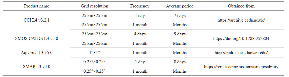
The European Space Agency Climate Change Initiative (ESA CCI) SSS products are produced by merging three satellite SSS based on optimal interpolation (OI), including SMOS Level 2 products, the SMAP Level 2 v4.0 products, and Aquarius Level 3 v5.0 products. The latest version of the ESA CCI products is v3.21 and there are two Level 4 datasets: the 7-day running means at one-day time sampling and the monthly products (Boutin et al., 2021). Both of them have a horizontal resolution of 25 km. The time range of CCI products is from January 2010 to December 2019.
2.1.2 SMOSThe SMOS SSS L3 v5 products are obtained from the Centre Aval de Traitement des Données (CATDS), this fifth version data used an improved ' de-biasing' technique to correct systematic biases and decrease biases in very variable regions as well as in noisy regions (e.g., high latitudes, radio frequency interference (RFI) contaminated areas) with a resolution of 25 km (Boutin et al., 2018). Two SMOS L3 SSS products are used in this study: the 9-day running means at 4-day time sampling and the monthly products. The time range of SMOS products is from January 2010 to December 2019.
2.1.3 AquariusThe monthly Aquarius SSS L3 v5.0 products are the final version of the Aquarius data (Kao et al., 2018) with a spatial resolution of 1°×1°. This version of data was released by the Aquarius Project in December 2017. The time range of Aquarius products is from August 2011 to May 2015.
2.1.4 SMAPThe SMAP SSS L3 v4.0 products are distributed by the Remote Sensing Systems (RSS). The Version 4.0 salinity products are distributed in two different spatial resolutions: 40 and 70 km. The 70-km data are obtained by smoothing the 40-km product using a simple near-neighbor averaging scheme over 9 cells (8 adjacent and the center cell itself) and should be regarded as the standard product for scientific applications in the open-ocean (Menezes, 2020). Without specifying, the SMAP L3 v4.0 product used in this article refers to the 70-km products. There are two datasets: the 8‐ day running means at 1-day time sampling and the monthly products. Both of them have a horizontal resolution of 0.25°×0.25°. The time range of SMAP products is from April 2015 to December 2019.
2.2 In-situ gridded SSS fieldsThe EN 4.2.1 monthly gridded data, which is used to validate the satellite SSS products, is provided by the Met Office Hadley Center (Good et al., 2013). This dataset is based on in-situ temperature and salinity profiles, including Global Temperature and Salinity Profile Program (GTSPP), World Ocean Database 2013 (WOD13), Argo data, and so on (details available at https://www.metoffice.gov.uk/hadobs/en4/download-en4-2-1.html). The EN 4.2.1 monthly mean 1°×1° salinity data is computed based on objective analysis using in-situ profiles from various observation after quality control including Argo, CTD, glider, and drifting buoys. The topmost layer is chosen to compare with the monthly satellite SSS products, which is 5.02 m below the sea surface.
2.3 Argo profileIn this study, SSS observations from Argo profiles in the SCS (0°–25°N, 100°E–125°E) for the period of January 2010 to December 2019, were selected from the global ocean Argo temperature-salinity profiles data set (http://www.geodoi.ac.cn/WebCn/doi.aspx?Id=1823) that is produced by China Argo Real-time Data Center and has been used to correct temperature and salinity drift (Liu and Wei, 2021). Argo profiles with quality control flags with values of 1 (good) for depth, position, date, salinity, and depth shallower than 10 m were selected. 6 000 and 60 profiles were selected after quality control (QC) for the period of January 2010–December 2019 in the SCS. In the 10-year profiles after QC, about 4.4% of SSS measurements were shallower than 2 m, 44.8% between 2 and 5 m, and 50.8% between 5 and 10 m. The selected Argo SSS measurements mainly distributed in the north of 10°N (Fig. 1a) and the number of measurements varied from year to year, the maximum and minimum numbers of measurements occurred in 2013 and 2019, with the corresponding numbers of 1 626 and 25, respectively (Fig. 1b).

|
| Fig.1 Spatial distribution of Argo profile SSS observations (a) and the number of Argo profile SSS observations per year (b) in the SCS during 2010–2019 |
For the first time, the European Space Agency (ESA) Climate Change Initiative Sea Surface Salinity (CCI+SSS) project combined SMOS, Aquarius, and SMAP measurements to generate Level 4 (L4) gridded SSS products. Due to better sampling and improved spatial resolution of salinity characteristics, the merged SSS products reduced the noise of satellite SSS (Boutin et al., 2021). Figure 2 shows the SSS maps from SMOS, Aquarius, SMAP, CCI, and EN 4.2.1 in April 2015. The spatial pattern of four satellites SSS data agrees with the EN 4.2.1 data in many details, such as the relatively high salinity areas located in the northern SCS and relatively low salinity areas found in the Beibu Gulf of China, and the Gulf of Thailand. In addition, the mesoscale features around tropical river plumes (e.g., the Mekong River Offshore), frontal regions (e.g., Luzon Strait) are well captured by satellites SSS data. It is worth noting that the satellite SSS are somewhat saltier than the EN 4.2.1 SSS in the southern SCS.

|
| Fig.2 The sea surface salinity maps of SMOS (a), Aquarius (b), SMAP (c), CCI (d), and EN 4.2.1 (e) monthly data of April 2015 in the South China Sea |
The period of each satellite data is different, so we use the same period for the comparison. The monthly averaged differences between the satellite products and EN 4.2.1 gridded data over the SMOS plus Aquarius data time periods (Fig. 3a–c) and the SMOS plus SMAP data periods (Fig. 3d–f) are shown in Fig. 3, while Fig. 4a–b displays the zonal average of SSS difference in the SCS. Overall, CCI and SMOS values are generally smaller than in-situ measurements in the north of 10°N and larger than in-situ measurements in the south of 10°N over both Aquarius and SMAP period, while Aquarius and SMAP values are smaller than in-situ measurements over the most of the SCS, especially in the northern SCS. The Version 5.0 SMOS is closer to the in-situ measurements than the previous version data because the latest SMOS used an improved "de-biasing" technique to correct systematic biases. The obvious negative biases of Aquarius and SMAP, which were observed near the coastline and in the shelf seas in the northern SCS, are likely to result from the strong radio frequency interference (Zeng et al., 2014). Owning to filter RFI contaminated measurements, CCI shows relatively less deviations near the coastline and in the shelf seas than Aquarius and SMAP (Boutin et al., 2021). From Fig. 4a–b, the zonal average biases of CCI and SMOS are closer to zero, while the zonal average biases of Aquarius and SMAP change from positive to negative and gradually increase with latitude from southern SCS to northern SCS. It should be noted that the zonal average biases of CCI and SMOS over the SMOS plus Aquarius (Fig. 4a) and the SMOS plus SMAP (Fig. 4b) data time periods is consistent in the south of 15°N, while slightly different in the north of 15°N. The zonal average biases of CCI and SMOS over the SMAP data period (Fig. 4b) are almost all negative in the north of 15°N. In contrast, the zonal average biases of CCI and SMOS over the Aquarius data period (Fig. 4a) changed from negative to positive in the north of 15°N. This suggests that the different length of time of the satellite data used as a sample have an effect on the distribution of the zonal average biases.

|
| Fig.3 The difference maps between CCI (a), SMOS (b), Aquarius (c) and monthly EN 4.2.1 data over the Aquarius data time periods (from August 2011 to May 2015), and CCI (d), SMOS (e), SMAP (f) and monthly EN 4.2.1 data over the SMAP data periods (from April 2015 to December 2019) |

|
| Fig.4 Zonal average of difference over the Aquarius data periods (from August 2011 to May 2015) (a) and SMAP data periods (from April 2015 to December 2019) (b) |
Overall, Fig. 3 shows that the satellite results are generally fresher in north of 10°N and saltier in south of 10°N. These discrepancies may be due to differences in depths of measurements (satellite: several centimeters near the surface; in-situ data: 2–10 m below the surface). Qi et al. (2022) also found that satellite observations are relatively saltier in the south of the SCS and fresher in the northern part compared with WOA18 SSS data. Furthermore, the in-situ observations used in the monthly EN 4.2.1 are mainly from Argo floats in the SCS (Bao et al., 2019; Liu et al., 2022). The Argo data are mainly distributed in the north of 10°N of the SCS (Fig. 1a) except for the coastline and in the shelf seas, and an insufficient of data measured may lead to large error in the southern SCS.
Figure 5 shows the distribution of the mean root-mean-square deviation (RMSD) of satellite SSS products with respect to the monthly EN 4.2.1 data over the SMOS plus Aquarius data time periods (Fig. 5a–c) and the SMOS plus SMAP data time periods (Fig. 5d–f). The RMSD is calculated as 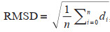

|
| Fig.5 The root-mean-square deviations (RMSDs) of CCI (a), SMOS (b), Aquarius (c) over the Aquarius data periods (from August 2011 to May 2015), and CCI (d), SMOS (e), SMAP (f) over the SMAP data time periods (from April 2015 to December 2019) with the monthly EN 4.2.1 data |
The results show that the satellite SSS products agree well with the in-situ data (RMSD < 0.4) in the SCS except the regions along the coast and in the shelf seas where the large RMSD values can be observed (RMSD > 0.6). Overall, the RMSD of CCI is lower than that of a single satellite no matter in the SMOS plus Aquarius period or in the SMOS plus SMAP period. It is worth noting that the RMSD of CCI is not as good as that of a single satellite data in some regions. The most obvious is the RMSD of SMAP (Fig. 5f) is smaller than that of CCI data (Fig. 5e) in the central SCS, the possible reasons for this is that the SMAP data we used is Version 4.0, the major change is an improved land correction compared with Version 3.0 (Boutin et al., 2021). The SMOS product used to derive CCI L4 SSS is non-corrected for land contamination. The SMOS and Aquarius data are in general more affected by RFI than SMAP data in coastlines and marginal seas (Reul et al., 2020). In addition, the CCI merging methodology have not considered correcting Aquarius SSS for systematic latitudinal seasonal biases before merging with SMOS SSS, and systematic differences arising from the radiative transfer models (Boutin et al., 2021).
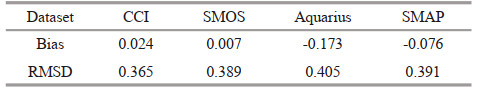
Figure 6a shows the time series of the mean differences between each of the four satellite SSS products and in-situ gridded data. Except that the differences of Aquarius are always less than zero, the other products yield time series oscillating around zero, especially CCI and SMOS. The time series of the RMSD between each of the four satellite SSS products and in-situ data are shown in Fig. 6b. During the period with SMOS data only (from January 2010 to July 2011), the RMSD of CCI is small than SMOS, while during the period with SMOS plus Aquarius data (from August 2011 to May 2015), the RMSD of CCI SSS products is gradually closer to SMOS, even larger than SMOS. This is mainly because of considering a correction for seasonal latitudinal biases for SMOS, while not considering correcting Aquarius SSS for systematic latitudinal seasonal biases before merging with SMOS (Boutin et al., 2021). During the period with SMOS plus SMAP measurements (from September 2015 to December 2019), the RMSD of CCI trends to increase compared with the SMOS only period and the SMOS plus Aquarius period. It is noted that the RMSD of CCI and SMOS seems to have a seasonal peak from July to November, indicating that the SMOS retrieval may be affected by some seasonal processes (Bao et al., 2019). Table 2 shows the statistical differences between each of the four satellite SSS products and EN 4.2.1 data. The RMSD of satellite SSS are smaller than 0.4 except for Aquarius, and the RMSD of CCI (0.365) is the lowest among the four satellite products.

|
| Fig.6 The monthly time series of the bias (a) and root-mean-square deviation (RMSD) (b) between four satellite SSS products and EN 4.2.1 data |
In order to study the quality of satellite SSS products in different regions of the SCS, four regions are selected (Fig. 7). These regions include the Zhujiang (Pearl) River estuary (ZRE) region (112°E–115°E, 20°N–23°N) and the Mekong River offshore (MR) region (105°E–109°E, 8°N–12°N) being adjacent to the land with the intense river runoff, and the Beibu Gulf (BBG) region (105°E–110°E, 18°N–23°N), and the Gulf of Thailand (GT) region (100°E–105°E, 5°N–15°N) representing semi-enclosed gulf.

|
| Fig.7 Regions selected out, including the Beibu Gulf (BBG) region (105°E–110°E, 18°N–23°N), the Zhujiang River estuary (ZRE) region (112°E–115°E, 20°N–23°N), the Mekong River offshore (MR) region (105°E–109°E, 8°N–12°N), and the Gulf of Thailand (GT) region (100°E–105°E, 5°N–15°N) |
The RMSDs of the four satellite products in the four selected regions show obvious seasonal changes, which is corresponding to the characteristics of the monsoon system in the SCS with the obvious period of the summer monsoon and the winter monsoon (Hu et al., 2000). In the summer season (from May to September), extensive precipitation and associated river runoff are produced by warm and humid winds (Yi et al., 2020), the dilution of freshwater results in low SSS values. In Beibu Gulf, the RMSDs of CCI, SMOS, and SMAP are found to be the largest during August (Fig. 8a) as the salinity reaches a minimum value when precipitation is the highest in August-September (Chen et al., 2019). In the ZRE, the RMSD of CCI, SMOS, Aquarius, and SMAP are found to be the largest during June (Fig. 8b) mainly attributing to the contribution from river runoff due to the heavy rainfalls during the Pre-Flood Season of South China (from April 1 to June 30). The largest RMSD of the four satellite products in the Mekong River offshore is found in September–October (Fig. 8c) since the extensive precipitations during the wet season (June–November) of the Mekong River Basin (https://www.mrcmekong.org/about/mekong-basin/climate/) dilute the freshwater plumes in the Mekong River outflow. The largest RMSD of the four satellite products in the Gulf of Thailand is very similar to that in the Mekon River offshore (Fig. 8d), possibly as a result of the contribution of the Mekong River runoff (Yi et al., 2020).

|
| Fig.8 Monthly averaged root-mean-square difference (RMSD) of four satellite products in four regions a. Beibu Gulf (BBG) region; b. Zhujiang River estuary (ZRE) region; c. Mekong River offshore (MR) region; d. Gulf of Thailand (GT) region. |
In addition, in the near coastal areas and the shelf seas, RFI errors, insufficient in-situ data, and land contamination are also sources of errors. On one hand, the RFI contamination results in low SSS values, predominantly contributing to the large negative bias of Aquarius and SMAP (Fig. 3c–d) near the coastline and in the shelf seas in the northern SCS. On the other hand, the limited number of in-situ data sampling in coastal areas (Fig. 1a), leading to large errors in monthly in-situ gridded products. As a result, using the gridded data to validate satellite data in these places possibly causes additional errors.
3.2 Comparison with Argo profilesThe Argo SSS observations are used to validate the satellite products on a weekly time scale. The accuracies of CCI, SMOS, and SMAP are mainly evaluated because Aquarius ceased operation in June 2015. For each Argo profile SSS observation, we perform spatio-temporal matching with the satellite observation. As the daily gridded CCI, SMOS, and SMAP is the running mean of seven-, nine-, and eight-day respectively; therefore, we select Argo profiles in the time interval of 7, 9, and 8 days across the satellite SSS acquisition date respectively, and then interpolate the daily SSS on the position of the selected Argo profile. After collocation, there are 35 975 collected pairs formed for the CCI and 11 199 collected pairs for the SMOS during Jan. 2010–Dec. 2019, while 9 838 collected pairs for the SMAP during Apr. 2015–Dec. 2019 in the SCS.
The results of the comparison between satellite SSS and Argo SSS observations are displayed in Fig. 9. Overall, the satellite SSS and Argo SSS observations are uniformly distributed on both sides of Y=X, predominately occurring in the salinity range of 33–34. CCI and SMAP are more concentrated on both sides of Y=X than SMOS, which the correlation coefficient between CCI and Argo observation is higher than that for SMOS but slightly lower than SMAP (Fig. 10). However, compared with Argo observation, the RMSD of CCI is smaller than SMOS and slightly smaller than SMAP. Meanwhile, all the three satellite products show negative biases (Fig. 10), and the RMSD of CCI weekly time scale products with 0.295 is the lowest among the three satellite products.

|
| Fig.9 Scatter plots of collocated CCI (a), SMOS (b), and SMAP SSS (c) versus Argo SSS observation in the SCS for period from 1 January 2010 to 31 December 2019 for CCI and SMOS, 1 April 2015 to 31 December 2019 for SMAP The black lines show a 1꞉1 relationship. The color represents the data density of scattered points. |

|
| Fig.10 Bar diagrams of statistics for comparisons between satellite product (CCI, SMOS, SMAP) and Argo floats over the entire SCS |
Figure 11 displays the histogram of bias and RMSD between Argo floats and satellite SSS products. The values of bias and RMSE for CCI were scaled in order to show within the same plot. The biases of the three satellite products distributed mainly between -0.8 and 0.8, and the most frequent occurrence is around zero (Fig. 10a). The RMSDs of CCI and SMAP are distributed mainly between 0.1 and 0.8, the number of floats decreases significantly with the increase of RMSD, while the RMSD of SMOS distributes at 0.1–1, the number of floats decreases slowly with the increase of RMSD (Fig. 10b).

|
| Fig.11 Histogram of bias and root-mean-square deviation between CCI, SMOS, SMAP, and Argo floats from 1 January 2010 to 31 December 2019 a. Bias; b. RMSD. |
This paper presented a systematic analysis of the accuracies of the four different SSS products from three salinity satellites missions (SMOS, Aquarius, and SMAP) in the SCS based on in-situ salinity measurements over 2010–2019. The SSS products include CCI L4 data (monthly and 7 days), SMOS CATDS L3 data (monthly and 9 days), Aquarius V5.0 L3 data (monthly), and SMAP L3 data (monthly and 8 days).
The accuracies of four different SSS products are assessed by comparing and analyzing with in-situ gridded data and Argo floats. Comparison with monthly EN 4.2.1 gridded data shows that the satellite results are generally fresher in north of 10°N and saltier in south of 10°N. The RMSDs of CCI, SMOS, Aquarius, and SMAP are 0.365, 0, 389, 0.405, and 0.391 in the SCS, respectively. The merged CCI is of the highest accuracy in the SCS. The RMSDs of SMOS, Aquarius, and SMAP are close, and the SMOS CATDS takes a slight advantage in accuracy in contrast with Aquarius and SMAP. Large errors can be found in the regions along with the coast and in the shelf seas, suggesting the impact of RFI and land contamination should be taken seriously into account and need to further improve the retrieval algorithms in these regions. Comparison of satellite SSS products with Argo floats indicates satellite products are able to capture the variety of salinity on weekly time scales. The merged CCI weekly products with lower RMSD (0.295) perform better than single satellite data (SMOS: 0.517, SMAP: 0.297) in the SCS. On average, whether compared with in-situ grid data or Argo floats, the CCI have the smallest RMSD among the four satellite products, which illustrates the improved accuracy of merged CCI with respect to the individual satellite data in the SCS.
Overall, the accuracy of CCI is better than that of individual satellites in the SCS. However, due to the continuous improvement of the inversion algorithms, the accuracy of individual satellite product has also been improved in some scenarios. For example, in the central SCS, the accuracy of SMAP is slightly higher than that of CCI due to its improved land correction. Secondly, for coastal and the southern SCS where the Argo profiles are less frequently sampled, its accuracy still needs to be verified using other observations, and should be used with caution. There is still a room for the validation of CCI L4 SSS in the SCS. On one hand, the comparison of in-situ and satellite measurements remains to be improved. It is necessary to strengthen the collection of other in-situ observations (e.g., marine stations, mooring platforms, and vessels) to compare them with CCI, especially in the coastal and southern part of the South China Sea, where Argo sampling is scarce. On the other hand, Comparison with some other satellite SSS data, such as HY-2A, is also worth considering. This will better reflect the advantages of CCI-SSS.
As one of the largest marginal seas, the RFI and land contamination in the SCS are relatively serious, predominantly leading to the higher RMSD observed than the open ocean. Thus, a systematic evaluation of SSS retrieval is suggested before research application in marginal seas and coastal regions. Meanwhile, for the first time, the CCI SSS product, which merged three satellite sensors SSS measurements over a decade, is likely to be a better choice to describe and apprehend the SCS SSS variability in future studies.
5 DATA AVAILABILITY STATEMENTThe datasets generated during and/or analyzed during the current study are available from the corresponding author on reasonable request.
Akhil V P, Vialard J, Lengaigne M, et al. 2020. Bay of Bengal Sea surface salinity variability using a decade of improved SMOS re-processing. Remote Sensing of Environment, 248: 111964.
DOI:10.1016/j.rse.2020.111964 |
Balaguru K, Chang P, Saravanan R, et al. 2012. Ocean barrier layers' effect on tropical cyclone intensification. Proceedings of the National Academy of Sciences of the United States of America, 109(36): 14343-14347.
DOI:10.1073/pnas.1201364109 |
Bao S L, Wang H Z, Zhang R, et al. 2019. Comparison of satellite-derived sea surface salinity products from SMOS, Aquarius, and SMAP. Journal of Geophysical Research, 124(3): 1932-1944.
DOI:10.1029/2019JC014937 |
Boutin J, Chao Y, Asher W E, et al. 2016. Satellite and in situ salinity: understanding near-surface stratification and subfootprint variability. Bulletin of the American Meteorological Society, 97(8): 1391-1407.
DOI:10.1175/BAMS-D-15-00032.1 |
Boutin J, Reul N, Koehler J, et al. 2021. Satellite-based sea surface salinity designed for ocean and climate studies. Journal of Geophysical Research, 126: e2021JC017676.
DOI:10.1029/2021JC017676 |
Boutin J, Vergely J L, Marchand S, et al. 2018. New SMOS sea surface salinity with reduced systematic errors and improved variability. Remote Sensing of Environment, 214: 115-134.
DOI:10.1016/j.rse.2018.05.022 |
Boyer T P, Levitus S. 2002. Harmonic analysis of climatological sea surface salinity. Journal of Geophysical Research, 107(C12): 8006.
DOI:10.1029/2001JC000829 |
Chen B, Xu Z X, Ya H Z, et al. 2019. Impact of the water input from the eastern Qiongzhou Strait to the Beibu Gulf on Guangxi coastal circulation. Acta Oceanologica Sinica, 38(9): 1-11.
DOI:10.1007/s13131-019-1472-2 |
Droghei R, Buongiorno Nardelli B, Santoleri R. 2018. A new global sea surface salinity and density dataset from multivariate observations (1993-2016). Frontiers in Marine Science, 5: 84.
DOI:10.3389/fmars.2018.00084 |
Du Y, Zhang Y H. 2015. Satellite and Argo observed surface salinity variations in the tropical Indian Ocean and their association with the Indian Ocean dipole mode. Journal of Climate, 28(2): 695-713.
DOI:10.1175/JCLI-D-14-00435.1 |
Good S A, Martin M J, Rayner N A. 2013. EN4: Quality controlled ocean temperature and salinity profiles and monthly objective analyses with uncertainty estimates. Journal of Geophysical Research, 118(12): 6704-6716.
DOI:10.1002/2013JC009067 |
Hackert E, Ballabrera-Poy J, Busalacchi A J, et al. 2011. Impact of sea surface salinity assimilation on coupled forecasts in the tropical Pacific. Journal of Geophysical Research, 116(C5): C05009.
DOI:10.1029/2010JC006708 |
Hlywiak J, Nolan D S. 2019. The influence of oceanic barrier layers on tropical cyclone intensity as determined through idealized, coupled numerical simulations. Journal of Physical Oceanography, 49(7): 1723-1745.
DOI:10.1175/JPO-D-18-0267.1 |
Hu J Y, Kawamura H, Hong H S, et al. 2000. A review on the currents in the South China Sea: seasonal circulation, South China Sea warm current and Kuroshio intrusion. Journal of Oceanography, 56(6): 607-624.
DOI:10.1023/A:1011117531252 |
Kao H Y, Lagerloef G S E, Lee T, et al. 2018. Assessment of Aquarius sea surface salinity. Remote Sensing, 10(9): 1341.
DOI:10.3390/rs10091341 |
Li C J, Zhao H, Li H P et al. 2015. Assessment of SMOS and Aquarius/SAC-D salinity data accuracy in the South China Sea: three statistical methods. In: Proceedings of 2015 IEEE International Geoscience and Remote Sensing Symposium. IEEE, Milan, Italy. p. 954-957, https://doi.org/10.1109/IGARSS.2015.7325925.
|
Li Y H, Liu T T, Shang S L. 2016. On the performance of Aquarius sea surface salinity V4 product in the South China Sea. Journal of Xiamen University (Natural Science), 55(4): 522-530.
(in Chinese with English abstract) |
Liu H, Wei Z X. 2021. Intercomparison of global sea surface salinity from multiple datasets over 2011-2018. Remote Sensing, 13(4): 811.
DOI:10.3390/rs13040811 |
Liu Y X, Cheng L J, Pan Y Y, et al. 2022. Climatological seasonal variation of the upper ocean salinity. International Journal of Climatology, 42(6): 3477-3498.
DOI:10.1002/joc.7428 |
Lukas R, Lindstrom E. 1991. The mixed layer of the western equatorial Pacific Ocean. Journal of Geophysical Research, 96(S01): 3343-3357.
DOI:10.1029/90JC01951 |
Menezes V V. 2020. Statistical assessment of sea-surface salinity from SMAP: Arabian Sea, Bay of Bengal and a promising red sea application. Remote Sensing, 12(3): 447.
DOI:10.3390/rs12030447 |
Pang S S, Wang X D, Foltz G et al. 2020. Modulation of June rainfall in India by winter salinity barrier layer in the Bay of Bengal, https://doi.org/10.21203/rs.3.rs-102922/v1.
|
Qi J F, Du Y, Chi J W, et al. 2022. Impacts of El Niño on the South China Sea surface salinity as seen from satellites. Environmental Research Letters, 17(5): 054040.
DOI:10.1088/1748-9326/ac6a6a |
Qin S S, Wang H, Zhu J, et al. 2020. Validation and correction of sea surface salinity retrieval from SMAP. Acta Oceanologica Sinica, 39(3): 148-158.
DOI:10.1007/s13131-020-1533-0 |
Ren Y Z, Dong Q, He M X. 2015. Preliminary validation of SMOS sea surface salinity measurements in the South China Sea. Chinese Journal of Oceanology and Limnology, 33(1): 262-271.
DOI:10.1007/s00343-014-3338-5 |
Reul N, Grodsky S A, Arias M, et al. 2020. Sea surface salinity estimates from spaceborne L-band radiometers: an overview of the first decade of observation (2010-2019). Remote Sensing of Environment, 242: 111769.
DOI:10.1016/j.rse.2020.111769 |
Stammer D, Martins M S, Köhler J, et al. 2021. How well do we know ocean salinity and its changes?. Progress in Oceanography, 190: 102478.
DOI:10.1016/j.pocean.2020.102478 |
Vinogradova N, Lee T, Boutin J, et al. 2019. Satellite salinity observing system: recent discoveries and the way forward. Frontiers in Marine Science, 6: 243.
DOI:10.3389/fmars.2019.00243 |
Wang X X, Yang J H, Zhao D Z, et al. 2013. Assessment of Aquarius/SAC-D salinity data accuracy in the South China Sea. Journal of Tropical Oceanography, 32(5): 23-28.
(in Chinese with English abstract) |
Yan Y F, Li L, Wang C Z. 2017. The effects of oceanic barrier layer on the upper ocean response to tropical cyclones. Journal of Geophysical Research, 122(6): 4829-4844.
DOI:10.1002/2017JC012694 |
Yi D L, Melnichenko O, Hacker P, et al. 2020. Remote sensing of sea surface salinity variability in the South China Sea. Journal of Geophysical Research, 125(12): e2020JC016827.
DOI:10.1029/2020JC016827 |
Zeng L L, Liu W T, Xue H J, et al. 2014. Freshening in the South China Sea during 2012 revealed by Aquarius and in situ data. Journal of Geophysical Research, 119(12): 8296-8314.
DOI:10.1002/2014JC010108 |
Zhu J S, Huang B H, Zhang R H, et al. 2014. Salinity anomaly as a trigger for ENSO events. Scientific Reports, 4(1): 6821.
DOI:10.1038/srep06821 |