 2023, Vol. 41
Institute of Oceanology, Chinese Academy of Sciences
Article Information
- LI Zhao, ZHANG Yingxin, SONG Shuqun, LI Caiwen
- Impacts of algal blooms on sinking carbon flux and hypoxia off the Changjiang River estuary
- Journal of Oceanology and Limnology, 41(6): 2180-2196
- http://dx.doi.org/10.1007/s00343-022-2278-8
Article History
- Received Jul. 14, 2022
- accepted in principle Sep. 15, 2022
- accepted for publication Oct. 13, 2022


2 CAS Key Laboratory of Marine Ecology and Environmental Sciences, Institute of Oceanology, Chinese Academy of Sciences, Qingdao 266071, China;
3 Marine Ecology and Environmental Science Laboratory, Laoshan Laboratory, Qingdao 266237, China;
4 University of Chinese Academy of Sciences, Beijing 100049, China;
5 Center for Ocean Mega-Science, Chinese Academy of Sciences, Qingdao 266071, China
Estuaries, the critical transition zones linking land and the sea, are important for resource repository, nutrient cycling, and economic development (Bianchi, 2010; Bauer et al., 2013; Cloern et al., 2014). Under the interplay between climate changes and anthropogenic activities, estuaries are more vulnerable to environmental pressures and become ecologically fragile in recent years (Regnier et al., 2013; Wei et al., 2021). Similar to most estuaries in the world, the Changjiang (Yangtze) River estuary (CE) and its adjacent waters is characteristic of high biological production and suffers from intensive eutrophication, harmful algal blooms (HAB), and seasonal hypoxia (Chai et al., 2006; He et al., 2013; Wang at al., 2016a; Wei et al., 2021).
Phytoplankton is the main source of primary production and plays a key role in marine ecosystems (Falkowski and Woodhead, 1992; Paerl et al., 2003; Hays et al., 2005). Systematic and long-term investigations have been conducted in the CE and its adjacent waters since 1980s, and substantial data on the phytoplankton community have been accumulated (Li and Mao, 1985; Luan et al., 2008; Song et al., 2017). The most dominant phytoplankton groups in this area were diatoms and dinoflagellates, and their relationships with environmental conditions were also analyzed (Chiang et al., 1999, 2004; Guo et al., 2014). It has been shown that Changjiang Diluted Water (CDW) regulates the distribution of phytoplankton assemblage, especially diatoms. Harmful algal blooms posed multiple threats to the structure and function of the ecosystem (Glibert et al., 2005), and increased in the CE and its adjacent waters in terms of both number and scale (Zhou et al., 2008). Both Prorocentrum donghaiense and Skeletonema costatum were the most frequent bloom-forming algae in spring and summer (Zhou et al., 2008). The occurrences of diatom and dinoflagellate blooms were impacted by Changjiang River discharge and Kuroshio intrusion (Zhou et al., 2019).
As a result of eutrophication, hypoxia has become a severe ecological phenomenon in the CE and its adjacent waters in recent decades (Zhu et al., 2011; Wang et al., 2016a; Chi et al., 2020). Wang et al. (2012) reported that the hypoxia began in late spring and early summer, became severe in August, then eased in the following months, and disappeared completely in winter. Hypoxia covered an area of up to 15 400 km2 off the CE in the summer of 2006 (Zhu et al., 2011). It is generally accepted that seasonal stratification and organic matter decomposition were essential factors contributing to the formation of hypoxia in this area (Wang et al., 2016a; Zhu et al., 2016). Due to the increased riverine nutrient loads, higher primary productivity resulted in more organic matter transported to the surface sediment, thus facilitating the deficit of oxygen through its further decomposition (Lohrenz et al., 2008; Zhou et al., 2008; Grenz et al., 2010). For the CE and its adjacent waters, analysis is restricted duo to the lack of straightforward evidence, thus we need to assess sinking carbon flux of phytoplankton and its contribution to the formation of hypoxia.
In this study, 10 multidisciplinary cruises were conducted in the CE and its adjacent waters from February 2015 to January 2016. The monthly variations in species composition, cell abundance, carbon biomass, and sinking rates of phytoplankton, were assessed comprehensively, as well as their association with temperature, salinity, nutrient conditions, and water masses. Further, the impacts of algal blooms on sinking carbon flux and hypoxia were evaluated quantitatively, to depict the formation of seasonal hypoxia.
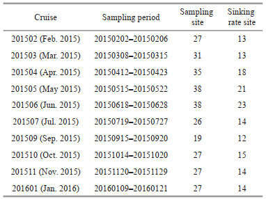
2 MATERIAL AND METHOD 2.1 Study area and cruise informationThe CE and its adjacent waters are affected by a complex hydrological system, mainly including CDW, the Coastal Currents (CC) along Chinese mainland, the Taiwan Warm Current (TWC) from Taiwan Strait, and the Nearshore Kuroshio Branch Current (NKBC) (Su, 1998). The CDW forms stratified and turbid plumes, with a basin area of 1.8×10⁶ km2 and a large load of terrestrial materials (nutrients and organic matter) from the drainage basin, especially in summer (Zhang et al., 2007). The inshore and offshore branches of the TWC flow northeasterly when the southwest monsoon prevails. The NKBC from northeast of Taiwan, China, flows northeastward along the 100-m isobaths and can reach 31°N (Yang et al., 2012). Generally, the study area is strongly influenced by the East Asian Monsoon climate and variable environmental conditions, which lead to spatial-temporal heterogeneity in the phytoplankton assemblage (Zhu et al., 2009; Song et al., 2017). From February 2015 to January 2016, 10 cruises were carried out in the CE and its adjacent waters, with the assistance of the R/Vs Kexue 3 and Beidou. The locations of sampling stations are presented in Fig. 1, but the actual sampling stations in different sampling periods varied as displayed in the following figures. The cruise information is listed in Table 1. In addition, Transect zb was selected to study and illustrate the vertical distribution of major phytoplankton groups according to the location of harmful algal blooms.

|
| Fig.1 Study area and location of sampling stations |
Water temperature, salinity, and density were determined by shipborne CTD probes (SBE 917, Sea-Bird Scientific, USA). Discrete water samples were collected from the standard layer (if the distance between the bottom layer and the standard layer is less than 5 m, only the bottom layer was collected), using 12-L Niskin bottles (KC-Denmark Ltd., Denmark) at each station. Dissolved oxygen (DO) was analyzed onboard using the Winkler titration method. Inorganic nutrients (NO3-N, NO2-N, NH4-N, PO4-P, and Si(OH)4-Si) were measured using an autoanalyzer (San++, SKALAR, the Netherlands), and chlorophyll-a (Chl-a) concentrations were determined using a fluorometer (Trilogy, Turner, USA) according to Strickland and Parsons (1972).
Phytoplankton assemblage analysis was conducted according to Utermöhl (1958). Seawater samples (250 mL) from each layer were preserved with buffered formalin (final concentration 5%). Subsamples of 10–25 mL were concentrated in a chamber (Hydrobios, Germany) for 24 h, then identified and counted under an inverted microscope (IX71, Olympus, Japan) at ×200 or ×400 magnification (Tomas, 1997).
Phytoplankton cell volume was calculated from the linear dimensions with their geometric models (Sun and Liu, 2003). More than 30 individual cells were measured for linear dimensions to avoid bias. Carbon content and equivalent spherical diameter (ESD) of phytoplankton cells was then converted from cell volume according to Eppley et al. (1970):
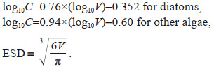
In which C is the cell carbon content in pg C/cell, and V is the cell volume in μm3. When calculating the ESD of chain-forming species, V is calculated as the volume of the chain rather than the single cell.
Phytoplankton sinking rates were measured by the SETCOL method (Bienfang, 1981). Three Plexiglas columns (height: 0.348 m, volume: 460 mL) were conducted. The columns were filled with surface seawater and capped, then settled undisturbed in the dark for an hour. After the incubation was terminated, the upper, middle, and bottom layers of the SETCOL compartments were drained in sequence by taps through the wall. Using the phytoplankton biomass (Chl a) before and after incubation in the three compartments, the phytoplankton community sinking rates were calculated based on the formula:
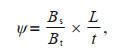
where ψ is the sinking rate; Bs is the biomass in the bottom compartment after incubation; Bt is the total biomass in the column; L is the height of the column; t is the settling interval.
The sinking carbon flux of phytoplankton (F) was calculated according to the following formula:

where ψ and C are the average sinking rate and average carbon biomass of phytoplankton in water column, respectively. Phytoplankton carbon biomass was calculated as the sum of the product of cell carbon content of each phytoplankton species and its cell abundance.
2.3 Data analysis and statistical analysisThe diversity of the phytoplankton assemblage was demonstrated by the Shannon-Weiner diversity index (log2H′) (Shannon and Wiener, 1949; Sun and Liu, 2003). Based on McNaughton index (Y), the dominant phytoplankton species were calculated using the following formula:
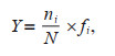
where ni is the sum of cell abundance for species i in all samples; N is the sum of cell abundance for all species, and fi is the frequency of occurrence for species i in all samples.
The cell abundance threshold of bloom was determined based on the China's National Marine Industry Standard (No. HY-T069-2005): Technical Specification for Red Tide Monitoring.
One-way analysis of variance (ANOVA) was applied to calculate correlation in different sampling sites, with the significant level of 0.05. The relationships between phytoplankton abundance and environmental factors were calculated by Pearson's correlation analysis. Spearman's rho correlation analysis was conducted between the zonal positions of low DO and high Chl a. All statistical tests were conducted with the SPSS (Version 20.0 for windows, SPSS Inc., USA). The correlations between sinking carbon flux of phytoplankton and DO at the bottom layer were plotted in Origin software (Version 2021b, OriginLab, USA).
3 RESULT 3.1 Environmental variable 3.1.1 Monthly variationThe variations of the environmental conditions in the CE and its adjacent waters during 10 cruises are shown in Supplementary Fig.S1. The seawater temperature ranged from 6.24 to 28.15 ℃. It was highest in July, with average of 27.09±0.70 ℃, and lowest in February, with average of 11.17±3.22 ℃. The surface temperature increased in the offshore direction, and presented relatively high values in the southeast of the study area. The salinity ranged from 14.41 to 34.45 in gradient. In the upper layer, the salinity increased in the offshore direction, indicating the expansion of CDW (S < 30). In February and March, the CDW distributed in the west of 122.5°E. The scope expanded to 123°E in April began to shrink in May, and was restricted to the coastal waters throughout the summer. In September, the trend of extension appeared again. The CDW dwindled in nearshore waters from October to January. In the bottom layer, the salinity was low at the nearshore stations and increased gradually offshore. Notably, the intrusion of NKBC (S > 34.3) significantly influenced the Zhejiang coastal area (> 50 m) from April.
The monthly average of dissolved inorganic nitrogen (DIN) in whole water column, ranging from 8.65 to 17.29 μmol/L, increased from February (10.33±6.48 μmol/L) to July (17.29±20.06 μmol/L), then decreased in September. The phosphate concentration presented high level and slight spatial fluctuations. The average of phosphate in whole water column was lowest in June, and highest in November. The variation of silicate in whole water column was similar to that of DIN, with the monthly average ranging from 11.02 to 22.24 μmol/L.
The Chl-a concentration in whole water column varied from 0.17 to 20.44 μg/L, and were relatively higher from late spring to early autumn. The Chl-a concentration ranged from 0.50 to 14.05 and 0.14 to 20.44 μg/L, on average of 3.55±3.10 and 4.46± 5.11 μg/L in April and July, respectively. Chl-a concentration in nine stations, i.e., za6a and DH5-4 in April, zb12a in June, zb7, 12300-3, 12300-4, and za1 in July, 12300-5 and 12250-4 in October, exceeded 10 μg/L, indicating the outbreak of algal blooms.
3.1.2 Vertical profileVertical profiles of temperature, salinity, DIN, phosphate, and silicate along Transect zb are shown in Fig. 2 to demonstrate the vertical distributions of main environmental variables in 10 cruises. In February, the environmental variables showed vertical homogeneity because of strong vertical mixing (Fig. 2, 1.a.–1.e.). In March, high temperature (> 16 ℃) and salinity (> 34) were observed at the bottom near 123°E (Fig. 2, 2.a.–2.e.). It indicated the intrusion of NKBC. The DIN and phosphate showed high concentrations in the low salinity area. In April, the CDW expanded eastward and induced the stratification of water column. The intrusion of NKBC was strengthened as well. As a result, the bottom water presented higher temperature (17–18 ℃), salinity (> 34), and phosphate concentration (Figs. 2, 3.a.–3.e.). During May–July, the CDW receded, while the NKBC expanded upward and westward, occupying the whole water column to the east of station zb12a in July (Figs. 2, 4.a.–6.e.). Meanwhile, the surface temperature increased and formed stratification. Phosphate showed a high concentration in the bottom. In addition, the TWC occurred in May when surface layer temperature was > 20 ℃ and salinity > 33.5. In September, the CDW expanded eastward, while the vertical profiles of temperature, DIN, and phosphate were similar to that in July (Fig. 2s, 7.a.–7.e.). In October, NKBC, TWC, and CDW withdrew (Figs. 2, 8.a.–8.e.). As a result, the concentrations of DIN and phosphate decreased. In November and January, the NKBC was not observed in Transect zb, and vertical mixing was strengthened again (Figs. 2, 9.a.–10.e.).

|
| Fig.2 Vertical profiles of temperature (℃), salinity, DIN (μmol/L), phosphate (μmol/L), and silicate (μmol/L) along Transect zb 1-10 represent month; a–e represent environmental variables. |
In total, 265 phytoplankton species (in 5 phyla and 94 genera) were identified during sampling period. A total of 27 taxa appeared in all cruises and 46 taxa in nine cruises. The total species number was relatively high from April to October (Fig. 3). Diatoms (Bacillariophyta) and dinoflagellates (Dinophyta), which accounted for 63.78% and 33.21% of total species respectively, were the dominant groups. Both of them showed the highest number of species in April. The numbers of species representing the Chlorophyta, Chrysophyta, and Cyanophyta were low on all cruises.

|
| Fig.3 Variation of phytoplankton species during 10 cruises |
The top 5 dominant phytoplankton species are listed in Supplementary Table S1. Chain-forming diatoms, such as Paralia sulcate (Ehrenberg) Cleve, Lauderia annulate Cleve, Cerataulina pelagica (Cleve) Hendey, Pseudo-nitzschia pungens (Grunow ex Cleve) G. R. Hasle, and Melosira moniliformis (O. F. Müller) C. Agardh, were the most common dominant species in the study area, while dinoflagellates dominated the assemblage in spring and early summer (from April to July). A benthic diatom Paralia sulcata, was the most dominant species in February and March. A HAB dinoflagellate Prorocentrum donghaiense D. Lu, became the most dominant species in April, and Lauderia annulata and Ceratanlina pelagica were the most dominant species in May and June, respectively. A small single-cell diatom Cylindrotheca Closterium (Ehrenberg) Reimann & J. C. Lewin, represented the highest dominance in July. The most dominant species in September and October, respectively, were the chain-forming diatoms Pseudo-nitzschia pungens and Melosira moniliformis. The only dominant species belonging to Cyanophyta, Trichodesmium thiebautii Gomont ex Gomont dominated in November and could indicate the intrusion of TWC. In January, Lauderia annulata became the most dominant species again. Compared to that in May, Lauderia annulata showed a higher appearance frequency and lower proportion of abundance.
The distributions of Shannon-Wiener index (H′) at surfaces are shown in Supplementary Fig. S2. In February and March, H′ ranged from 0.71 to 3.78, with the relatively low value located in the northeast study area. In April, H′ ranged from 0.08 to 3.71, presented low value in the southeast study area, with the minimum value at DH5-4. From May to July, H′ formed high patches in the south study area. From September to November, H′ increased in the offshore direction. In January, H′ ranged from 0.64 to 3.35, with the relatively high value in the middle of the study area.
3.2.3 Cell abundanceBased on the analysis of 295 sampling sites during 10 cruises, the variation of phytoplankton abundance off the Changjiang River estuary (CE) and its adjacent waters is shown in Fig. 4. The phytoplankton abundance ranged from 0.07×10³ to 5 132.62× 10³ cells/L, on average of (36.62±233.46)×103 cells/L. It was relatively low and showed slight fluctuations in spring and winter. The maximum of total abundance appeared in July and the minimum of total abundance in November. Dinoflagellates were abundant in only spring and early summer, while diatoms determined the total abundance, especially in winter.

|
| Fig.4 The monthly variation of phytoplankton abundance in sampling sites during 10 cruises Data were transformed logarithmically [lg(x)] before analyses. |
The horizontal distributions of surface phytoplankton abundance are shown in Fig. 5. In February and March, diatoms dominated the distribution of phytoplankton abundance, which increased in the offshore direction. In April, both diatoms and dinoflagellates presented high abundances in the southeast study area. The dinoflagellate abundance ranged from 0.36×10³ cells/L to 1 599.73×10³ cells/L. In May, the surface abundance decreased, especially in the southeast study area, where the dinoflagellates presented very low abundances. In June, the surface phytoplankton formed two high-abundance patches around stations 12300-5 and 12300-1, respectively. The northern patch was attributed to dinoflagellates, while the southern patch was attributed to diatoms. In July, the surface abundance was higher in the southwest study area. In September, the surface abundance was high in the southwest study area. In October, diatoms dominated the distribution of phytoplankton abundance as well. The higher abundances of both phytoplankton and diatoms were distributed in the middle of the study area, while dinoflagellates presented higher abundance in the northern area. In November–December, high abundances appeared in the northern part of the study area.

|
| Fig.5 The horizontal distribution of surface phytoplankton abundance (×103 cells/L) in the study area a. total phytoplankton; b. diatom; c. dinoflagellate. |
The vertical profiles of phytoplankton abundance along Transects zb are shown in Fig. 6. The Chl a and phytoplankton presented low values and small spatial variations in February and March. In April, high abundances and Chl-a concentration appeared in the upper layers. Chl-a concentration exceeded 10 μg/L at the surface layer of station DH5-4 (14.05 μg/L). In June, the Chl-a concentration was higher in the upper layer. Both in July and October, patches of high abundance appeared at stations zb7 and zb12a respectively. In November and January, phytoplankton was distributed homogeneously throughout the water column along Transect zb.

|
| Fig.6 Vertical profiles of Chl a (μg/L), total phytoplankton abundance (×103 cells/L), diatom abundance (×103 cells/L), and dinoflagellate abundance (×103 cells/L) along Transect zb 1-10 represent the Survey month; a. Chl a; b. total phytoplankton abundance; c. diatom abundance; d. dinoflagellate abundance. |
The relationship between environmental variables and phytoplankton abundance are shown in Fig. 7. Phytoplankton abundance presented significantly negative correlations with temperature in March, May, and November (P < 0.05). Significantly negative correlations were observed between phytoplankton abundance and salinity in July and October (P < 0.05), and no significant correlation was observed in other months. Phytoplankton abundances correlated negatively with nutrient concentration in April (P < 0.05), while positively in July. No obvious correlation was observed between phytoplankton abundances and any nutrient concentration in fall and winter.

|
| Fig.7 Pearson's correlation analysis between phytoplankton cell abundance and environmental parameters during the 10 cruises *: P < 0.05; **: P < 0.01. |
The distributions of phytoplankton carbon biomass at surfaces are shown in Fig. 8. Carbon biomass in February and March was evenly distributed and relatively low. In April, carbon biomass was higher in the southeast of study area, and reached the peak of 921.80 mg C/m3 at station zb12a. In May, the patch with higher carbon biomass appeared in the south of study area, closer to Zhejiang coast than in April. The maximum value of 337.60 mg C/m3 located at station za6c. In June and July, carbon biomass exceeded 100 mg C/m3 at most stations, and presented peak value 20 484.40 mg C/m3 at station zb7 in July. Generally, it decreased in the offshore direction. In September, the distribution of carbon biomass was similar to that in May, with the highest value at station za6c (279.61 mg C/m3). In October, phytoplankton carbon biomass was relatively high in the middle of the survey area. However, the carbon biomass was relatively low in November and January.

|
| Fig.8 Horizontal distribution of DO (mg/L) at the bottom layer and phytoplankton carbon biomass (mg C/m3) at the surface Circles represent the phytoplankton carbon biomass. The contour represents the DO concentration (obtained from the study by Li et al. (2018)). |
The phytoplankton carbon flux in the study area was roughly estimated by using the sinking rates and carbon biomass of water column at each station. The variation of carbon flux is shown in Fig. 9. In October, the carbon flux ranged from 0.70 to 464.10 mg C/(m2·d), reaching the highest average of 78.90±119.34 mg C/(m2·d), followed by June when the carbon flux ranged from 1.44 to 360.91 mg C/(m2·d) on average of 63.16±99.98 mg C/(m2·d). In April, the phytoplankton carbon flux ranged from 0.33 to 111.46 mg C/(m2·d) on average of 20.90±28.90 mg C/(m2·d), a result of a bloom of P. donghaiense. It is noteworthy that the average phytoplankton carbon flux in October was 3.8 times higher than that in April, even though the phytoplankton cell abundance were approximately equal in two months. Generally, the carbon flux was relatively low in winter.

|
| Fig.9 Variation of phytoplankton carbon flux (a); variation of DO at the bottom layer (b); relationship between phytoplankton carbon flux and DO at the bottom layer (c) All data were transformed logarithmically [ln(x)] before analyses in Fig. 9c. |
Bloom of P. donghaiense (dinoflagellate) and C. closterium (diatom) were observed in spring and summer, respectively. In April, P. donghaiense presented high cell abundance (1 599.73×10³ cells/L) at the surface of station DH5-4, contributing more than 90% of phytoplankton cell abundance. In July, the phytoplankton cell abundance was high in the southwest of the study area and showed maximum (5 132.62×10³ cells/L) at 10-m layer of station zb7, where cell abundance of C. closterium exceeded 106 cells/L.
During the dinoflagellate bloom, the intensified NKBC intrusion increased the temperature and salinity below 20 m, and brought high-salinity water to the bottom of the southern study area (Figs. 10, 1.a. & 1.b.). In contrast, a strong pycnocline appeared around the 20-m layer during the diatom bloom (Figs. 10, 2.a. & 2.b.). The water columns both above and below the pycnocline were weakly stratified. The increasing stratification at nearshore stations above 20 m could be a result of the net air-sea heat flux into the ocean and the extension of TWC in the summer.

|
| Fig.10 The vertical profiles of temperature (℃) and salinity, the distributions of surface phytoplankton carbon biomass (mg C/m3) and bottom DO (mg/L) 1.a.–1.f.: dinoflagellate bloom; 2.a.–2.f.: diatom bloom. The circles represent the phytoplankton carbon biomass. |
The maximum value of Chl a during the diatom bloom was 20.44 μg/L, higher than dinoflagellate bloom (14.05 μg/L). The relatively high value region of Chl a was located in high values of temperature and salinity during dinoflagellate bloom. While high values of Chl a were associated with low salinity during the diatom bloom, which was influenced by TWC in the nearshore. The diatom bloom accumulated more carbon biomass than dinoflagellate bloom. During diatom blooms, as chain-forming species such as C. closterium and Rhizosolenia acuminata (Péragallo) Gran showed high cell abundances, the phytoplankton carbon biomass reached 20 484.4 mg C/m3. While, phytoplankton dominated by small-sized species such as P. donghaiense and the phytoplankton carbon biomass was 1 605.26 mg C/m3 during dinoflagellate bloom. The water-column-integrated phytoplankton carbon biomass was 49 471.87 mg C/m2 at diatom bloom station, and 29 853.03 mg C/m2 at dinoflagellate bloom station. The DO of the bottom layer during algal blooms and the following months are shown in Fig. 8. The minimum value of DO during the dinoflagellate bloom (6.36 mg/L) was higher than that during the diatom bloom (4.08 mg/L). Moreover, low DO zones (< 3.0 mg/L) appeared in August, which was associated with the area with higher carbon biomass during diatom bloom.
4 DISCUSSIONHypoxia and HAB off the CE and its adjacent waters is a prominent phenomenon in recent decades (Zhao and Guo, 2011; Wei et al., 2015). Previous studies have identified the importance of phytoplankton in the formation of hypoxia (Chi et al., 2020). Moreover, diatom-dominated phytoplankton community has higher sinking rates than the dinoflagellate-dominated community, and transports more particulate organic matter to the bottom during algal blooms (Li et al., 2018). In the present study, diatoms and dinoflagellates are two major phytoplankton groups and formed blooms in July (P. donghaiense) and April (C. closterium), respectively. Phytoplankton carbon flux was estimated and showed a significantly negative relationship with DO concentration in the bottom. The results suggest that the export of primary production from surface waters provided the materials for organic matter decomposition and DO depletion in the bottom off the Changjiang River estuary.
4.1 Effect of environmental factors on phytoplankton assemblagesThe phytoplankton assemblage is known to be influenced by environmental variables, including temperature, salinity, and nutrients (Wang, 2002; Ershadifar et al., 2020; Gerhard et al., 2022). Different phytoplankton assemblage and species demand different optimum environmental conditions. In April, the phytoplankton assemblage was dominated by P. donghaiense at optimum temperature and salinity of 17 ℃ and 32, respectively. It is known that P. donghaiense shows strong competitive ability with other phytoplankton species under low phosphate concentrations (Wang and Huang, 2003). In April, an increase in salinity, temperature, and nutrient concentrations with high N꞉P ratio (28.58–44.77) could be suitable for P. donghaiense blooms in offshore area. Overall, the relatively high nutrients concentrations were inshore and the high P. donghaiense abundance was in offshore, reflected in the negative correlation between phytoplankton abundance and nutrients. Some chain-forming diatoms such as P. sulcata dominated in three months (Supplementary Table S1). In July, diatoms dominated by C. closterium and M. moniliformis were positively correlated with nutrient concentrations; however, most of the chain-forming diatoms were not closely correlated with environmental variables in other months (Fig. 7). With the variation of environmental conditions, several phytoplankton species alternately dominated in the communities.
In some cases, the phytoplankton responds to certain environmental variables in one system, while in another, it might behave differently, thus leading to different optima and tolerances (Resende et al., 2005). In the CE and its adjacent waters, chain-forming diatoms constituted the background assemblage and could change into the dominant group when environmental conditions were suitable for their growth (Guo et al., 2014).
4.2 The relationship between phytoplankton carbon flux and the formation of hypoxiaThe seasonally low DO and hypoxia was reported in the bottom waters off the CE in 2015 (Li et al., 2018), and is shown in Figs. 8 & 9b. The DO concentration was closely correlated with the blooming and decomposition of phytoplankton. The zone of high phytoplankton carbon biomass in the upper layer tended consistent with low DO in bottom water. There was a significantly positive correlation between the latitudinal positions of DO minimum in the bottom anoxic zone and high Chl-a core in the surface layer in September and October (R=0.912, n=5, P < 0.05), thus demonstrating that the primary production was the main source of the organic matter in the bottom water.
The fate of phytoplankton-derived organic matter is largely determined by the dominant groups of the primary producers. It was found that the cells disintegrated in the water column before reaching the bottom water during a Peridiniella catenata (Levander) Balech (dinoflagellate) bloom. Phytoplankton cells deposited out of the water column rapidly due to fast sinking rates during diatom-dominated blooms and thus left less time for zooplankton and bacteria to decompose them (Passow, 1991; Heiskanen and Kononen, 1994). In the CE and its adjacent waters, Guo et al. (2016) found that the sinking rates of phytoplankton during a P. donghaiense bloom were significantly slower than during a Skeletonema dorhnii bloom. According to Li et al. (2018), diatom blooms contribute more particulate organic matter to the bottom waters than dinoflagellate blooms. Moreover, hypoxia in the near-bottom waters was correlated to the sinking of phytoplankton community dominated by diatoms in the upper layer of the study area.
Thus, to clarify the role of phytoplankton in the formation of hypoxia, the phytoplankton carbon flux was estimated. The bottom DO concentration displayed a significantly negative correlation with phytoplankton carbon flux (Fig. 9c). The decomposition of organic matter plays an important role in the formation of hypoxia in the study area (Chen et al., 2007; Zhu et al., 2011). The changes in the DO content are closely related to the coupled process of organic matter decomposition and nutrient regeneration (Hsiao et al., 2014). In the study area, apparent oxygen utilization (AOU) displayed significant positive correlations with nitrate and phosphate, indicating that the regeneration of nutrients in the near-bottom waters was associated with high DO consumption, which contributed to hypoxia (Chi et al., 2017). In August, the biological silicon content of surface sediment was higher in station zb7, with the content more than 1.80% (Fan et al., 2019). Thus, phytoplankton carbon flux dominated by diatoms in June, July and October, provided the materials for organic matter decomposition and DO depletion in the bottom. Moreover, Wang et al. (2016b) suggested that the export of primary production was more important than the allochthonous input of organic matter for fueling DO depletion in bottom waters, based on the quantification of the δ13C value of remineralized organic carbon. These observations provided straightforward evidence for the source of organic matter for oxygen consumption in the study area. Zhu et al. (2013) reported that if only organic matter degradation and oxygen consumption are considered, it could then further be estimated that it would take 50–150 days to develop hypoxia after stratification prevails off the Changjiang estuary. Taken together, the patches of primary production lead to the discontinuous distribution of hypoxia.
4.3 The dinoflagellate and diatom bloomsOver the past decades, as HAB have become a serious ecological issue in coastal ecosystems around the world, the mechanisms and consequences of HAB studies have been studied (Anderson et al., 2008; Zhou et al., 2008, 2019; Shumway et al., 2018). In the study area, the diatom and the dinoflagellate blooms occur successively every year. The most frequent bloom-causing species was P. donghaiense, followed by S. costatum, Karenia mikimotoi (Miyake & Kominami ex Oda) Gert Hansen & Moestrup, and Chaetoceros curvisetus Cleve (Shen et al., 2011). During the P. donghaiense bloom in April, the whole water column of station DH5-4 was characterized by high cell abundance except in bottom layer. The appearance of the high phytoplankton abundance was associated with the intrusion of NKBC. During the C. closterium bloom in July, the phytoplankton mainly concentrated in the upper layer (above 20 m) influenced by CDW, and decreased rapidly with depth at station zb7 (Fig. 6, 6. c.). It can be seen that the occurrence of algal blooms was affected by the different water mass. Zhou et al. (2017) reported that the dinoflagellate bloom was more associated with the NKBC, while the CDW was more important for the diatom bloom. The NKBC could affect the dynamics of HAB by transporting tropical phytoplankton into the adjacent waters of CE (Zhao et al., 2019). The P. donghaiense in the Kuroshio Current can serve as an important population source for P. donghaiense blooms in the CE and its adjacent waters (Xu et al., 2021). In the present study, the P. donghaiense bloom in April was related to the intrusion of NKBC, and the C. closterium bloom in July was related to CDW.
Due to the differences of cell morphology, structure, and nutrition mode between diatoms and dinoflagellates, the bloom strategy and carbon biomass were also different. During dinoflagellate bloom, the P. donghaiense contributed over 88% of total phytoplankton abundance and resulted in the low diversity at station DH5-4. Several diatom species such as Rhizosolenia acuminate (H. Peragallo) H. Peragallo showed high cell abundances (> 105 cells/L) and increase the community diversity at station zb7 during diatom bloom. Many studies have revealed that dinoflagellate blooms present lower diversity than diatom blooms, and the allelopathic effect plays a significant role in regulating phytoplankton communities (Smayda and Reynolds, 2003). The allelopathic effect provides dinoflagellates a survival strategy for competing with other phytoplankton species (Smayda, 1997). In addition, Heil et al. (2005) reported that Prorocentrum minimum (Pavillard) J. Schiller was able to inhibit the growth of other phytoplankton species. During harmful algal blooms, phytoplankton carbon biomass was relatively high. When higher algal mass sank to the bottom and decomposed by microbial community eventually, low DO and even hypoxia formed in bottom waters (Fig. 9), which can be reflected by the higher concentrations of biogenic silicate in the hypoxic region (Fan et al., 2019).
Although coastal eutrophication has been widely accepted as a major factor contributing to the increasing HAB globally (Sommer et al., 2012), nutrient condition is not the only controlling factor affecting the distributions and dynamics of HAB. Given sufficient nutrients in the water column, many other variables could affect the formation and dynamics of HAB, such as temperature in the optimal algal growth range, and availability of light, transport of bloom-forming species from other regions into the blooming region, the existence of parasitic dinoflagellates and grazing pressure (Glibert et al., 2005; Li et al., 2014; Haraguchi et al., 2015; Zhou et al., 2019). Therefore, the formation of HAB is the result of the interaction of environmental variables rather than single one.
5 CONCLUSIONDiatoms and dinoflagellates were the dominant phytoplankton groups and formed HAB respectively in the CE and its adjacent waters in 2015. The variation of phytoplankton abundance showed a close relationship with the environmental conditions and the dominant species presented distinctive distribution patterns due to their inherent environmental adaptation. The CDW induced environmental gradients in the upper layer, such as salinity and nutritional condition, favoring the diatom bloom of C. closterium in July. The intrusion of NKBC influenced phytoplankton assemblages in offshore waters, resulting in the formation of P. donghaiense bloom. With the blooming and senescence of phytoplankton, low DO and hypoxia occurred in the bottom waters off the CE. The higher phytoplankton carbon biomass increased the downward carbon flux and provided the materials for DO depletion in the bottom. Besides, the sinking of algal mass is a complicated process; more investigations are needed to develop a comprehensive understanding of the inter-annual variation of phytoplankton carbon flux, such as filed time-series station works and long-term monitory integrated Marine Observing System.
6 DATA AVAILABILITY STATEMENTThe data is available on request from the corresponding author.
7 ACKNOWLEDGMENTThe data were generated with the help of Prof. Zhiming YU at IOCAS.
Electronic supplementary material
Supplementary material (Supplementary Figs.S1–S2 and Table S1) is available in the online version of this article at https://doi.org/10.1007/s00343-022-2278-8.
Anderson D M, Burkholder J M, Cochlan W P, et al. 2008. Harmful algal blooms and eutrophication: examining linkages from selected coastal regions of the United States. Harmful Algae, 8(1): 39-53.
DOI:10.1016/j.hal.2008.08.017 |
Bauer J E, Cai W J, Raymond P A, et al. 2013. The changing carbon cycle of the coastal ocean. Nature, 504(7478): 61-70.
DOI:10.1038/nature12857 |
Bianchi T S, Dimarco S F, Cowan Jr J H, et al. 2010. The science of hypoxia in the Northern Gulf of Mexico: a review. Science of the Total Environment, 408(7): 1471-1484.
DOI:10.1016/j.scitotenv.2009.11.047 |
Bienfang P K. 1981. SETCOL-a technologically simple and reliable method for measuring phytoplankton sinking rates. Canadian Journal of Fisheries and Aquatic Sciences, 38(10): 1289-1294.
DOI:10.1139/f81-173 |
Chai C, Yu Z M, Song X X, et al. 2006. The status and characteristics of eutrophication in the Yangtze River (Changjiang) estuary and the adjacent East China Sea, China. Hydrobiologia, 563(1): 313-328.
DOI:10.1007/s10750-006-0021-7 |
Chen C C, Gong G C, Shiah F K. 2007. Hypoxia in the East China Sea: one of the largest coastal low-oxygen areas in the world. Marine Environmental Research, 64(4): 399-408.
DOI:10.1016/j.marenvres.2007.01.007 |
Chi L B, Song X X, Yuan Y Q, et al. 2017. Distribution and key influential factors of dissolved oxygen off the Changjiang River Estuary (CRE) and its adjacent waters in China. Marine Pollution Bulletin, 125(1-2): 440-450.
DOI:10.1016/j.marpolbul.2017.09.063 |
Chi L B, Song X X, Yuan Y Q, et al. 2020. Main factors dominating the development, formation and dissipation of hypoxia off the Changjiang Estuary (CE) and its adjacent waters, China. Environmental Pollution, 265: 115066.
DOI:10.1016/j.envpol.2020.115066 |
Chiang K P, Chen Y T, Gong G C. 1999. Spring distribution of diatom assemblages in the East China Sea. Marine Ecology Progress Series, 186: 75-86.
DOI:10.3354/meps186075 |
Chiang K P, Chou Y H, Chang J, et al. 2004. Winter distribution of diatom assemblages in the East China Sea. Journal of Oceanography, 60(6): 1053-1062.
DOI:10.1007/s10872-005-0013-7 |
Cloern J E, Foster S Q, Kleckner A E. 2014. Phytoplankton primary production in the world's estuarine-coastal ecosystems. Biogeosciences, 11(9): 2477-2501.
DOI:10.5194/bg-11-2477-2014 |
Eppley R W, Reid F M H, Stickland J D H. 1970. Estimates of phytoplankton crop size, growth rate and primary production. Bulletin of the Scripps Institution of Oceanography of the University of California, 17: 33-42.
|
Ershadifar H, Koochaknejad E, Ghazilou A, et al. 2020. Response of phytoplankton assemblages to variations in environmental parameters in a subtropical bay (Chabahar Bay, Iran): harmful algal blooms and coastal hypoxia. Regional Studies in Marine Science, 39: 101421.
DOI:10.1016/j.rsma.2020.101421 |
Falkowski P G, Woodhead A D. 1992. Primary Productivity and Biogeochemical Cycles in the Sea. Plenum Press, New York. 43p.
|
Fan X, Cheng F J, Yu Z M, Song X X. 2019. The environmental implication of diatom fossils in the surface sediment of the Changjiang River estuary (CRE) and its adjacent area. Journal of Oceanology and Limnology, 37(2): 552-567.
DOI:10.1007/s00343-019-8037-9 |
Gerhard M, Schlenker A, Hillebrand H, et al. 2022. Environmental stoichiometry mediates phytoplankton diversity effects on communities' resource use efficiency and biomass. Journal of Ecology, 110(2): 430-442.
DOI:10.1111/1365-2745.13811 |
Glibert P M, Anderson D M, Gentien P, et al. 2005. The global, complex phenomena of harmful algal blooms. Oceanography, 18(2): 136-147.
DOI:10.5670/oceanog.2005.49 |
Grenz C, Denis L, Pringault O, et al. 2010. Spatial and seasonal variability of sediment oxygen consumption and nutrient fluxes at the sediment water interface in a sub-tropical lagoon (New Caledonia). Marine Pollution Bulletin, 61(7-12): 399-412.
DOI:10.1016/j.marpolbul.2010.06.014 |
Guo S J, Feng Y Y, Wang L, et al. 2014. Seasonal variation in the phytoplankton community of a continental-shelf sea: the East China Sea. Marine Ecology Progress Series, 516: 103-126.
DOI:10.3354/meps10952 |
Guo S J, Sun J, Zhao Q B, et al. 2016. Sinking rates of phytoplankton in the Changjiang (Yangtze River) estuary: a comparative study between Prorocentrum dentatum and Skeletonema dorhnii bloom. Journal of Marine Systems, 154: 5-14.
DOI:10.1016/j.jmarsys.2015.07.003 |
Haraguchi L, Carstensen J, Abreu P C, et al. 2015. Long-term changes of the phytoplankton community and biomass in the subtropical shallow Patos Lagoon Estuary, Brazil. Estuarine, Coastal and Shelf Science, 162: 76-87.
DOI:10.1016/j.ecss.2015.03.007 |
Hays G C, Richardson A J, Robinson C. 2005. Climate change and marine plankton. Trends in Ecology & Evolution, 20(6): 337-344.
DOI:10.1016/j.tree.2005.03.004 |
He X, Bai Y, Pan D, et al. 2013. Satellite views of the seasonal and interannual variability of phytoplankton blooms in the eastern China seas over the past 14 yr (1998-2011). Biogeosciences, 10(7): 4721-4739.
DOI:10.5194/bg-10-4721-2013 |
Heil C A, Glibert P M, Fan C L. 2005. Prorocentrum minimum (Pavillard) Schiller: a review of a harmful algal bloom species of growing worldwide importance. Harmful Algae, 4(3): 449-470.
DOI:10.1016/j.hal.2004.08.003 |
Heiskanen A S, Kononen K. 1994. Sedimentation of vernal and late summer phytoplankton communities in the coastal Baltic Sea. Archiv für Hydrobiologie, 131(2): 175-198.
DOI:10.1127/archiv-hydrobiol/131/1994/175 |
Hsiao S S Y, Hsu T C, Liu J W, et al. 2014. Nitrification and its oxygen consumption along the turbid Chang Jiang River plume. Biogeosciences, 11(7): 2083-2098.
DOI:10.5194/bg-11-2083-2014 |
Ichikawa H, Beardsley R C. 2002. The current system in the Yellow and East China Seas. Journal of Oceanography, 58(1): 77-92.
DOI:10.1023/A:1015876701363 |
Li C W, Song S Q, Liu Y, et al. 2014. Occurrence of Amoebophrya spp. infection in planktonic dinoflagellates in Changjiang (Yangtze River) Estuary, China. Harmful Algae, 37: 117-124.
DOI:10.1016/j.hal.2014.05.009 |
Li R X, Mao X H. 1985. Dinoflagellates in the continental shelf of the East China Sea. Donghai Marine Science, 3(1): 41-55.
(in Chinese with English abstract) |
Li Z, Song S Q, Li C W, et al. 2018. The sinking of the phytoplankton community and its contribution to seasonal hypoxia in the Changjiang (Yangtze River) estuary and its adjacent waters. Estuarine Coastal and Shelf Science, 208: 170-179.
DOI:10.1016/j.ecss.2018.05.007 |
Lohrenz S E, Redalje D G, Cai W J, et al. 2008. A retrospective analysis of nutrients and phytoplankton productivity in the Mississippi River plume. Continental Shelf Research, 28(12): 1466-1475.
DOI:10.1016/j.csr.2007.06.019 |
Luan Q S, Sun J, Song S Q, et al. 2008. Phytoplankton assemblage in Changjiang estuary and its adjacent waters in autumn, 2004. Advances in Marine Science, 26(3): 364-371.
(in Chinese with English abstract) |
Paerl H W, Valdes L M, Pinckney J L, et al. 2003. Phytoplankton photopigments as indicators of estuarine and coastal eutrophication. BioScience, 53(10): 953-964.
DOI:10.1641/0006-3568(2003)053[0953:PPAIOE]2.0.CO;2 |
Passow U. 1991. Species-specific sedimentation and sinking velocities of diatoms. Marine Biology, 108(3): 449-455.
DOI:10.1007/Bf01313655 |
Regnier P, Friedlingstein P, Ciais P, et al. 2013. Anthropogenic perturbation of the carbon fluxes from land to ocean. Nature Geoscience, 6(8): 597-607.
DOI:10.1038/Ngeo1830 |
Resende P, Azeiteiro U, Pereira M J. 2005. Diatom ecological preferences in a shallow temperate estuary (Ria de Aveiro, Western Portugal). Hydrobiologia, 544(1): 77-88.
DOI:10.1007/s10750-004-8335-9 |
Shannon C E, Weaver W. 1949. The Mathematical Theory of Communication. The University of Illinois Press, Urbana. 131p.
|
Shen L, Xu H P, Guo X L, et al. 2011. Characteristics of large-scale harmful algal blooms (HABs) in the Yangtze River estuary and the adjacent East China Sea (ECS) from 2000 to 2010. Journal of Environmental Protection, 2(10): 1285-1294.
DOI:10.4236/jep.2011.210148 |
Shumway S E, Burkholder J M, Morton S L. 2018. Harmful Algal Blooms: A Compendium Desk Reference. Wiley, New Jersey. 667p.
|
Smayda T J, Reynolds C S. 2003. Strategies of marine dinoflagellate survival and some rules of assembly. Journal of Sea Research, 49(2): 95-106.
DOI:10.1016/S1385-1101(02)00219-8 |
Smayda T J. 1997. Harmful algal blooms: their ecophysiology and general relevance to phytoplankton blooms in the sea. Limnology and Oceanography, 42(5part2): 1137-1153.
DOI:10.4319/lo.1997.42.5_part_2.1137 |
Sommer U, Adrian R, De Senerpont Domis L, et al. 2012. Beyond the Plankton Ecology Group (PEG) model: mechanisms driving plankton succession. Annual Review of Ecology, Evolution, and Systematics, 43(1): 429-448.
DOI:10.1146/annurev-ecolsys-110411-160251 |
Song S Q, Li Z, Li C W, et al. 2017. The response of spring phytoplankton assemblage to diluted water and upwelling in the eutrophic Changjiang (Yangtze River) Estuary. Acta Oceanologica Sinica, 36(12): 101-110.
DOI:10.1007/s13131-017-1094-z |
Strickland J D H, Parsons T R. 1972. A Practical Handbook of Seawater Analysis. Fisheries Research Board of Canada, Ottawa. p. 201-206.
|
Su J L. 1998. Circulation dynamics of the China Sea: north of 18°N. In: Robinson A R, Brink K H eds. The Sea. John Wiley and Sons Inc., New York. p. 483-505.
|
Sun J, Liu D Y. 2003. Geometric models for calculating cell biovolume and surface area for phytoplankton. Journal of Plankton Research, 25(11): 1331-1346.
DOI:10.1093/plankt/fbg096 |
The China's National Marine Industry Standard (No. HY-T069-2005): Technical Specification for Red Tide Monitoring. Standards Press of China, Beijing, China. p. 21.
|
Tomas C R. 1997. Identifying Marine Phytoplankton. Academic Press, New York. p. 1-858.
|
Utermöhl H. 1958. Zur vervollkommnung der quantitativen phytoplankton methodik. Mitteilingen der Internationalen Vereinigung fur Theoretische und Angewandte Limnologie, 9: 1-30.
|
Wang B D, Wei Q S, Chen J F, et al. 2012. Annual cycle of hypoxia off the Changjiang (Yangtze River) estuary. Marine Environmental Research, 77: 1-5.
DOI:10.1016/j.marenvres.2011.12.007 |
Wang H J, Dai M H, Liu J W, et al. 2016a. Eutrophication-driven hypoxia in the East China Sea off the Changjiang estuary. Environmental Science & Technology, 50(5): 2255-2263.
DOI:10.1021/acs.est.5b06211 |
Wang J H, Huang X Q. 2003. Ecological characteristics of Prorocentrum dentatum and the cause of harmful algal bloom formation in China sea. Chinese Journal of Applied Ecology, 14(7): 1065-1069.
(in Chinese with English abstract) |
Wang J H. 2002. Phytoplankton communities in three distinct ecotypes of the Changjiang Estuary. Journal of Ocean University of Qingdao, 32(3): 422-428.
(in Chinese with English abstract) |
Wang W T, Yu Z M, Song X X, et al. 2016b. The effect of Kuroshio Current on nitrate dynamics in the southern East China Sea revealed by nitrate isotopic composition. Journal of Geophysical Research: Oceans, 121(9): 7073-7087.
DOI:10.1002/2016JC011882 |
Wei Q S, Wang B D, Chen J F, et al. 2015. Recognition on the forming-vanishing process and underlying mechanisms of the hypoxia off the Yangtze River estuary. Science China Earth Sciences, 58(4): 628-648.
DOI:10.1007/s11430-014-5007-0 |
Wei Q S, Wang B D, Zhang X L, et al. 2021. Contribution of the offshore detached Changjiang (Yangtze River) diluted water to the formation of hypoxia in summer. Science of the Total Environment, 764: 142838.
DOI:10.1016/j.scitotenv.2020.142838 |
Xu L J, Yang D Z, Yu R C, et al. 2021. Nonlocal population sources triggering dinoflagellate blooms in the Changjiang Estuary and adjacent seas: a modeling study. Journal of Geophysical Research: Biogeosciences, 126(11): e2021JG006424.
DOI:10.1029/2021jg006424 |
Yang D Z, Yin B S, Liu Z L, et al. 2012. Numerical study on the pattern and origins of Kuroshio branches in the bottom water of southern East China Sea in summer. Journal of Geophysical Research: Oceans, 117(C2): C02014.
DOI:10.1029/2011jc007528 |
Zhang J, Liu S M, Ren J L, et al. 2007. Nutrient gradients from the eutrophic Changjiang (Yangtze River) Estuary to the oligotrophic Kuroshio waters and re-evaluation of budgets for the East China Sea Shelf. Progress in Oceanography, 74(4): 449-478.
DOI:10.1016/j.pocean.2007.04.019 |
Zhao L, Guo X. 2011. Influence of cross-shelf water transport on nutrients and phytoplankton in the East China Sea: a model study. Ocean Science, 7(1): 27-43.
DOI:10.5194/os-7-27-2011 |
Zhao Y, Yu R C, Kong F Z, et al. 2019. Distribution patterns of picosized and nanosized phytoplankton assemblages in the East China Sea and the Yellow Sea: implications on the impacts of Kuroshio intrusion. Journal of Geophysical Research: Oceans, 124(2): 1262-1276.
DOI:10.1029/2018jc014681 |
Zhou M J, Shen Z L, Yu R C. 2008. Responses of a coastal phytoplankton community to increased nutrient input from the Changjiang (Yangtze) River. Continental Shelf Research, 28(12): 1483-1489.
DOI:10.1016/j.csr.2007.02.009 |
Zhou Z X, Yu R C, Sun C J, et al. 2019. Impacts of Changjiang river discharge and Kuroshio intrusion on the Diatom and Dinoflagellate Blooms in the East China Sea. Journal of Geophysical Research: Oceans, 124(7): 5244-5257.
DOI:10.1029/2019jc015158 |
Zhou Z X, Yu R C, Zhou M J. 2017. Resolving the complex relationship between harmful algal blooms and environmental factors in the coastal waters adjacent to the Changjiang River estuary. Harmful Algae, 62: 60-72.
DOI:10.1016/j.hal.2016.12.006 |
Zhu J R, Zhu Z Y, Lin J, et al. 2016. Distribution of hypoxia and pycnocline off the Changjiang estuary, China. Journal of Marine Systems, 154: 28-40.
DOI:10.1016/j.jmarsys.2015.05.002 |
Zhu Z Y, Ng W M, Liu S M, et al. 2009. Estuarine phytoplankton dynamics and shift of limiting factors: a study in the Changjiang (Yangtze River) Estuary and adjacent area. Estuarine, Coastal and Shelf Science, 84(3): 393-401.
DOI:10.1016/j.ecss.2009.07.005 |
Zhu Z Y, Zhang J, Wu Y, et al. 2011. Hypoxia off the Changjiang (Yangtze River) Estuary: oxygen depletion and organic matter decomposition. Marine Chemistry, 125(1-4): 108-116.
DOI:10.1016/j.marchem.2011.03.005 |
Zhu Z Y, Zhang J, Wu Y, et al. 2013. Early degradation rate particulate organic carbon and phytoplankton pigments under different dissolved oxygen level off the Changjiang (Yangtze) River Estuary. Oceanologia et Limnologia Sinica, 44(1): 1-8.
(in Chinese with English abstract) |